AGV Network
Overview and Key Concepts
The AGV Network helps you to create travel paths while simulating automatic guided vehicles (AGVs) and other task executers.
The AGV module does not add its own AGV object type to the library. Instead you attach task executers to control points on an AGV network, and those task executers will travel using AGV-defined logic.
Events
Task executers who have been attached to an AGV network will have additional events that can be subscribed to with a process flow Wait For Event or Event-Triggered Source activity.
- OnStartTravel - Fired when the AGV starts a travel task.
- OnFinishTravel - Fired when the AGV finishes a travel task.
- OnPreAllocate - Fired just before the AGV attempts to allocate forward. This will either be followed by one or more OnAllocate events or by an OnAllocationFailed event if it was not able to allocate forward. Allocation happens either on pre-arrival to a control point or when trying to allocate an intersection point on an accumulating path.
- OnAllocate - Fired when a control point, control area, or accumulating path intersection point is allocated.
- OnAllocationFailed - Fired when the AGV fails to allocate forward and hence must stop and wait.
- OnDeallocate - Fired when the AGV deallocates a control point, control area, or accumulating path intersection point.
- OnAccumulationStop - Fired when the AGV hits its proximity stop threshold on an accumulating path and must stop.
- OnAccumulationResume - Fired when the AGV hits its proximity resume threshold on an accumulating path and can resume.
- OnPreArrival - Fired at an AGV's pre-arrival to a control point, i.e. the point at which the AGV would start to decelerate to stop at the control point if needed. OnPreArrival is fired prior the AGV allocating further ahead, or when the AGV starts decelerating to its final destination.
- OnArrival - Fired at an AGV's arrival at a control point, i.e. when the AGV has decelerated to stop at the control point, either because it could not allocate further ahead or if the control point is the final destination.
Statistics
AGVs can track the following statistics:
- BatteryLevel - The AGV's battery level, as a percentage between 0 and 100.
The AGV Types Tab
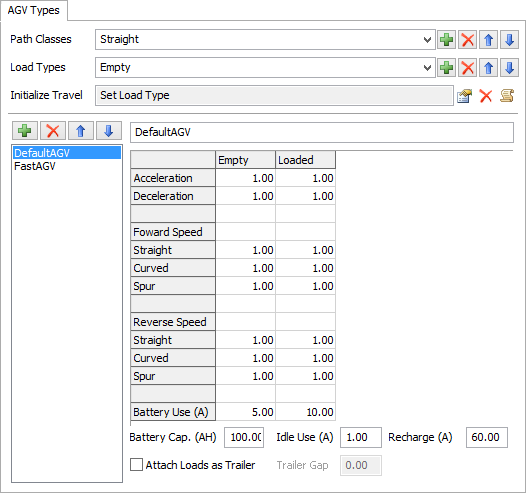
The AGV Types tab has the following properties:
You can get to the AGV Types page by right-clicking on a Path or Control Point and choosing AGV Network Properties.
Path Classes
Here you can add, remove, re-order and rename the set of Path Classes for the model. Path Classes are specifically used for breaking out AGV speeds by path. When you add a Path Class, a new speed row associated with that Path Class will be added to each AGV Type table for both forward and reverse speed.
Load Types
Here you can add, remove, re-order and rename the set of Load Types for the model. Load Types are a user-defined list defining categories for what an AGV is carrying. This allows you to break out AGV speeds by the AGV's current load.
Initialize Travel
This is a trigger that is fired at the beginning of each travel operation. The primary objective of this trigger is to set the AGV's current Load Type.
AGV Types List
Here you can add, remove, re-order and rename the list of AGV Types for the model.
AGV Type Spec Table
In the AGV Type Spec Table you define max speeds by Path Class, Load Type and AGV direction, as well as acceleration, deceleration and non-idle battery usage.
Battery Levels and Usage
Each AGV Type has a defined Battery Capacity (in Amp Hours), Idle Battery Usage (in Amps), and Recharge Rate (in Amps). Additionally, each AGV Type has a non-idle Battery Usage (in Amps) broken out by Load Type. Each AGV starts the simulation at its maximum battery capacity, and then will track its battery usage over the course of the simulation. Whenever it is idle, its Idle Battery Usage applies. Whenever it is doing a travel operation, its battery usage is based on its current Load Type. If you set the AGV to recharge, it will recharge at its recharge rate until it is full or it starts its next travel operation, whichever comes first. To query battery level, start a recharge, or manually set the battery level, etc., see the documentation for the agvinfo() command.
Attaching Trailers
You can also make the AGV attach loaded items as trailers to the AGV. This will make the loaded items trail behind the AGV on its path, instead of being carried on the AGV. Check the box Attach Loads as Trailer, and then define the Trailer Gap, which is the distance of the gap between the back of the AGV and the front of the trailing item.
Deceleration and End Speed
Usually when you give an AGV a task to travel to a destination, you will want the AGV to end that travel task fully decelerated to a stop. However, in some cases you may want to end a travel task while still moving, for example if you want to make dispatching decisions on-the-fly. In this case you can define a non-zero end speed for the travel task. Doing this will actually shift earlier the end time of the travel task, as well as the position of the AGV at the time it finishes. In other words, instead of ending on the destination control point while still moving, the travel task will end while the AGV is still approaching the control point, at the defined end speed. If you don't immediately give the AGV any subsequent travel tasks, then the AGV will decelerate down to stopped, arriving at the control point AFTER the travel task has finished. If, however, you immediately give the AGV a new travel task, it will continue to the new task, starting at the end speed of the previous task, traveling through the original destination control point.
The Way Points Tab
The Way Points tab has the following properties:
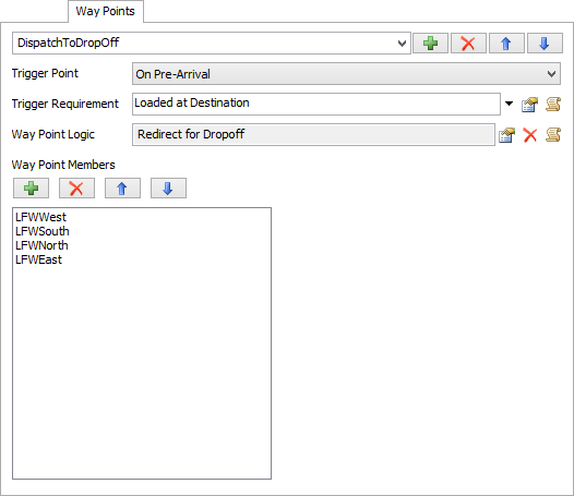
Way Points are used to define AGV control logic that will happen when an AGV passes over a control point. However, going forward we advise you to use process flow instead of Way Points for AGV control. FlexSim provides a template AGV control process flow, which can be used as a starting point for defining AGV control logic..
You can get to the Way Points page by right-clicking on a Path or Control Point and choosing AGV Network Properties.
Way Points List
Here you can add, remove, re-order, and rename each Way Point.
Trigger Point
This defines when to fire the Way Point Logic. Options are:
- On Pre-Arrival - The Way Point Logic will be fired at the point when the AGV would otherwise start to decelerate to stop at the Way Point.
- On Arrival - The Way Point Logic will be fired when the AGV arrives at the Way Point. Note that if the Trigger Requirement is met and this Trigger Point is chosen, the AGV will slow to a stop at this Way Point and then fire the Way Point, even if the Way Point is not the AGV's final destination. Hence if you don't want the AGV to slow to a stop, you should use On Pre-Arrival.
Trigger Requirement
A field that should return 1 if the Way Point should be fired, 0 if not.
Way Point Logic
The code for the Way Point.
Way Point Members
The list of Control Points that are part of this Way Point. Here you can add, remove and re-order the members list.
See Way Point Trigger Actions for more information.
The Control Point Connections Tab
The Control Point Connections tab has the following properties:
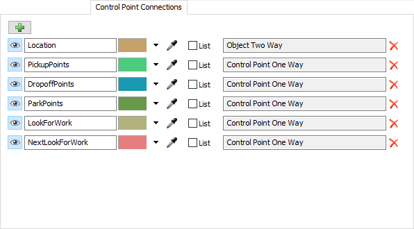
You can get to the Control Point Connections page by right-clicking on a Path or Control Point and choosing AGV Network Properties.
For each Control Point Connection, you can define whether or not its visible in the 3D view, and its color. You can also add, remove, and rename connections as needed.
Using Lists
If you check the List box for a connection, all of those connections in the model will be added to a global partitioned list. This allows you to easily define AGV control logic with a process flow. When an AGV arrives at a given destination, you can decide what to do by pulling from various list partitions associated with the AGV's current control point, such as, find a control point near here that has work that the AGV can do, or find a parking spot to go to, or continue to the next point to look for work. These operations can be done by pulling from the current control point's partition of the global list.
Connection Types
A Control Point Connection has one of three possible connection types:
- Control Point One-Way - This connection type means the connection is a one-way connection from one Control Point to another Control Point. In other words, when you make one of these connections from Control Point A to Control Point B, Control Point B will not have a connection back to Control Point A.
- Control Point Two-Way - This connection type means the connection is a two-way connection from one Control Point to another Control Point. In other words, when you add one of these connections from Control Point A to Control Point B, a connection from Control Point B back to Control Point A will automatically be created as well. When you add one of these connection types, you can make it so that the reverse connection (B back to A) connects back using the same connection type (the To Self option), or using a new connection type. Technically the two-way connection doesn't give you any added capability over the one-way because you can do this same functionality using one-way connections by manually adding one-way connections in both directions. However, this can save time in creating the connections if needed.
- Object Two-Way - This connection type represents a two-way connection from a Control Point to a model object. When you add one of these connections, the Control Point can accesss the object through that connection, and the object can access the control point through the same connection.
Using Connections
You can use Control Point connections through various trigger actions, such as Way Point trigger actions, or by manually accessing them with the cpconnection() command.
The Accumulation Types Tab
The Accumulation Types tab has the following properties:
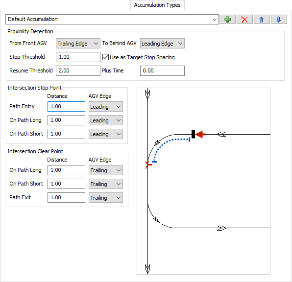
Accumulation Types let you define parameters for accumulating paths, i.e. paths on which AGVs will detect proximity and avoid collisions with each other.
You can get to the AGV Types page by right-clicking on a Path or Control Point and choosing AGV Network Properties.
Add, remove, rename and re-order Accumulation Types through the combobox and buttons at the top of the page.
To assign a path an Accumulation Type, click on the path, and in its Quick Properties on the right, choose the desired type from the Accumulation Type drop-down.
Proximity Detection
These properties define how two AGVs will detect proximity with each other while on a common accumulating path.
- From Front AGV Edge To Behind AGV Edge - This defines the AGV edges used to determine proximity. Usually this will be the default: Front AGV <Trailing Edge> to Behind AGV <Leading Edge>. This will evaluate the distance from the back of the AGV ahead to the front of the AGV behind. You could also choose something like Front AGV <Center> to Behind AGV <Center>, which would evaluate the distance from center to center.
- Stop Threshold - This is the proximity distance at which an AGV will go into a "proximity stop" state, and slow down to a stop.
- Use as Target Stop Spacing - If checked, then if an ahead AGV is stopped, the stop threshold defines the target stop spacing. Stopped AGVs will thus accumulate with this stop spacing. In other words, an AGV approaching a stopped AGV will begin decelerating to stop BEFORE the stop threshold (as a proximity distance) is breached. The AGV will instead start decelerating such that it comes to a stop with the stop threshold as its spacing behind the ahead AGV. In situations where both AGVs are still moving, the stop threshold will continue to be used in regular proximity detection.
- Resume Threshold - The proximity distance at which an AGV can resume its travel after going into a "proximity stop" state. The resume threshold must be greater than the stop threshold.
- Plus Time - An optional additional time, started when the Resume Threshold is reached, that the AGV will wait before resuming from a "proximity stop" state.
Intersections
When you define an Accumulation Type for a path, the AGV network will treat intersections on that path as allocations. Similar to the way AGVs must allocate Control Points and Control Areas, AGVs must allocate the intersection points on an accumulating path before proceeding past those intersection points. In the Accumulation Types page you define stop distances, which are distances before the intersection where the AGV must stop before an intersection point if the AGV cannot allocate it, as well as clear distances, which are distances after passing the intersection point where AGVs will release the intersection and allow other AGVs to claim it. Each of these distances are split out by whether the AGV is entering, exiting, or on the path. If already on a path or staying on a path, the distances are split out by the path geometry, i.e. whether or not the intersection branches out away from the AGV or toward it.
Intersection Stop Point
Here you define the stop distances for an intersection. For each distance, you define the distance itself as well as an AGV edge, which determine what part of the AGV should stop at the stop distance. Usually stop distances will be based on the leading edge of the AGV. When you click in a given field, the diagram on the right will display the distance / edge that you are defining, to help you figure out what exactly the field defines.
- Path Entry - This defines the stop distance and agv edge associated with entering a path.
- On Path Long - This defines the stop distance and agv edge associated with approaching an intersection when already on a path. It is the "long" stop distance because it will be applied to intersections that branch out toward the AGV, and thus require the AGV to stop farther away from the intersection point in order to provide room for merging AGVs.
- On Path Short - This defines the stop distance and agv edge associated with approaching an intersection when already on a path. It is the "short" stop distance because it will be applied to intersections that branch out away from the AGV, hence the AGV can stop closer to the intersection without causing issues.
Intersection Clear Point
Here you define the clear distances for an intersection. Like with stop distance, you define the distance itself as well as an AGV edge. Usually clear distances will be based on the trailing edge of the AGV. When you click in a given field, the diagram on the right will display the distance / edge that you are defining, to help you figure out what exactly the field defines.
- On Path Long - This defines the clear distance and agv edge associated with clearing an intersection when still on the path (not exiting). It is the "long" clear distance because it will be applied to intersections that branch out toward the clear point, and thus require the AGV to travel farther away from the intersection point before clearing it.
- On Path Short - This defines the clear distance and agv edge associated with clearing an intersection when still on the path (not exiting). It is the "short" clear distance because it will be applied to intersections that branch out away from the clear point, hence the AGV can clear it closer to the intersection point without causing issues.
- Path Exit - This defines the clear distance and agv edge associated with exiting a path.
Special Rules
There are a few special rules that apply to allocating intersection points.
- Pure On-Path Allocations - The AGV network tries to make basic proximity detection take precedence over intersection stop and clear points. Thus, if an AGV is already on a path and already has an AGV ahead of it for which it is detecting proximity, and if it is not exiting the path at that intersection, then the AGV will be allowed to allocate the intersection point before the ahead AGV has cleared it. Since it is already detecting proximity on the ahead AGV, it is OK to have a simultaneous allocation of the intersection point because the basic proximity detection will already avoid proximity errors.
- End-To-End Path Transfers - When transferring from the end of one path to the beginning of another path, the network still treats that as an "intersection" between two paths, i.e. it still requires an allocation of the intersection point. However, again if it can detect that, in transferring to the new path, the AGV will still be detecting proximity with the same AGV that it was detecting before the transfer, then it will go ahead and allow the intersection point to be allocated simultaneously by both AGVs, since the basic proximity detection will already prevent proximity errors. Note that this only applies to transfers between two paths of the same Accumulation Type. If the Accumulation Type is different, it will treat it like a regular intersection allocation.
Guidelines and Best Practices in Using Accumulation
Many users will see the option for accumulation and think this is the perfect solution for what they want to do. The truth, however, is that using accumulation, while making many simulation scenarios easier, can also introduce new complexities and potential problems. This doesn't mean you shouldn't use accumulation. Most encountered problems are easily fixed with the right know-how. Rather, you should just make sure you have a good understanding of how accumulation works before deciding to use accumulation.
The primary complexity with using accumulation is that it creates a new allocation scheme, one that is different than, but will operate in tandem with, the standard allocation scheme used for control points and control areas. Consequently, in some situations the two allocations schemes will "fight" with each other, and cause deadlock in the system. This is especially more probable in close-quarter intersection areas that use control areas to mutually exclude traffic.
An example problem situation is shown in the following figure.
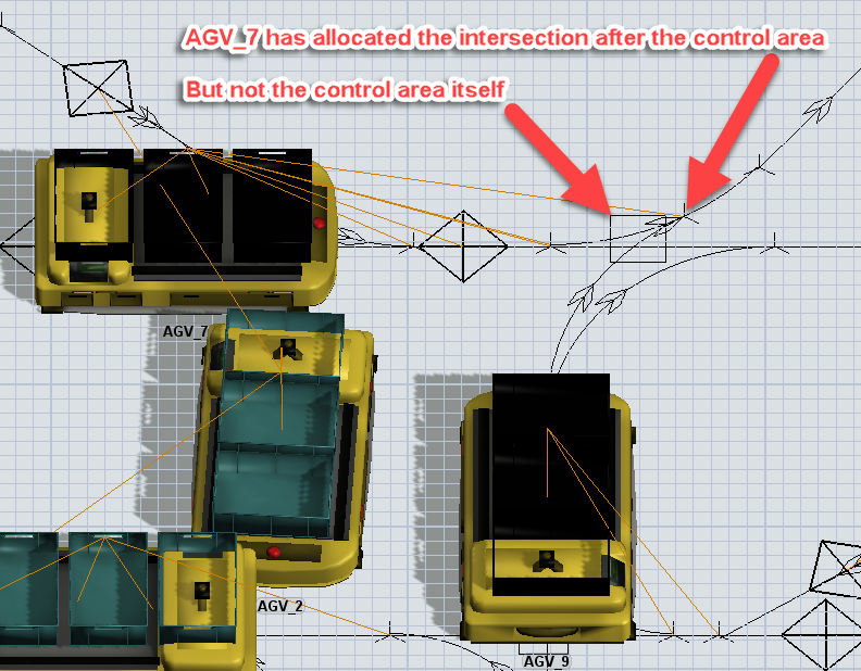
In this situation, AGV_7 has allocated the intersection after the control area, but has yet to allocate the control area itself. This creates a serious problem because AGV_9, the other AGV at the bottom center of the screen, will allocate the control area first. Then the two AGVs will get into a deadlock because AGV_7 can't allocate the control area owned by AGV_9, and AGV_9 can't allocate the intersection owned by AGV_7.
As mentioned before, this is caused because two different allocation schemes are in play here, namely the allocation of control areas vs. the allocation of intersections on accumulating paths. When allocating control areas, the AGV allocates when it pre-arrives at the previous control point. It will drive up to the closest control point, then allocate (in an all-or-nothing fashion) the next control point on its path, as well as all control areas on its path to that next control point. Thus the timing of when the AGV allocates the control area is based on the position of the control point leading up to the control area.
Accumulating intersection allocation, on the other hand, is determined based on the position of the intersection and the settings of the associated Accumulation Type, defined in AGV network properties. In the situation shown above, AGV_7 would use the "On Path Long" setting, whose default says the AGV should be able to stop with its leading edge at least one meter short of the intersection if it can't allocate that intersection. This determines the point at which the AGV will attempt to allocate the intersection.
In the example situation, AGV_7 allocates the intersection first because the control point is pretty close to the control area, so it reaches the point where it needs to allocate the intersection before it reaches the point where it needs to allocate the control area. On the other hand, AGV_9's control point is situated a little farther away from the control area, so it will allocate the control area before it allocates the intersection. This causes the deadlock.
Solutions
When encountering issues like this, there are two primary solutions you can try. First, you can create a special accumulation type that is specifically designed for close-quarter intersections. This accumulation type would ensure that control areas are always allocated before intersections. Here you would simply create a new accumulation type in the AGV network properties. Then for each intersection stop point, base it on the center of the AGV, with a distance of 0, meaning the AGV's center must stop 0 meters short of the intersection if the AGV can't allocate it. Once you've done that, make all the paths in that small area use that accumulation type.
The second solution to try is to simply not use accumulation in those close-quarter areas. Just go to each path in the intersection and make its accumulation setting "No Accumulation." This will make it so the control area is the sole mutually excluding element in the area. Then you don't have to worry about the right order of allocation. Here you'll want to make sure that the deallocation of the control area is not too early. You want the AGV to at least allocate the first intersection on an accumulating path ahead of it before it deallocates the control area. That shouldn't be too difficult. If it doesn't do it already, you can either lengthen the deallocation distance for that control area's deallocation type, or you can put down a control point at the beginning of the next accumulating path, then make the control area's deallocation type "Deallocate at Next Control Point."
As a general rule of thumb, accumulation works very well in areas of a model where there are long sections of path with relatively few intersections. On the other hand, in areas where there are lots of close-quarter intersections, it can be easier and less problematic to turn off accumulation, bound the areas with control points, and then limit traffic inside them with control areas.
The Deallocation Types Tab
The Deallocation Types tab has the following properties:
You can get to the Deallocation Types page by right-clicking on a Path or Control Point and choosing AGV Network Properties.
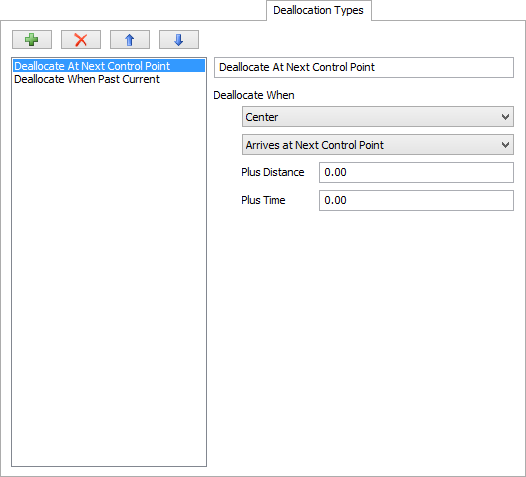
Deallocation Types List
Here you can add, remove, re-order and rename each Deallocation Type.
Edge Definition
This defines which "edge" of the AGV will determine the deallocation time. Options are:
- Center - Deallocation will be triggered when the AGV's center passes the given point.
- Trailing Edge - Deallocation will be triggered when the AGV's trailing edge passes the given point.
- Leading Edge - Deallocation will be triggered when the AGV's leading edge passes the given point.
Travel Point Definition
Defines the associated point on the path that determines deallocation time. Options are:
- Arrives at Next Control Point - Deallocation will be triggered when the AGV's defined edge arrives at the next Control Point. For Control Areas, this is the next Control Point after the path exits the Control Area.
- Passes Current Point - Deallocation will be triggered when the AGV's defined edge passes the current point. For Control Points this is the Control Point itself. For Control Areas, this is the point on the path where the AGV's defined edge exits the Control Area.
Plus Distance
This is an additional distance that will be added onto travel before deallocating the object.
Plus Time
This is an additional time to delay deallocation, after the defined edge has reached the travel point plus the distance.
The Visual Tab
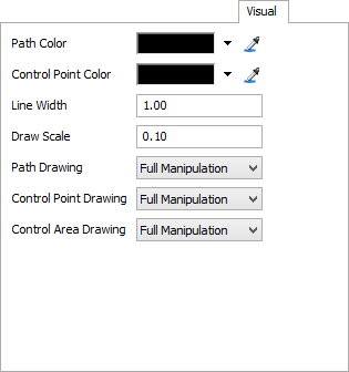
The Visual tab has the following properties:
You can get to the Visual page by right-clicking on a Path or Control Point and choosing AGV Network Properties.
Path Color
Defines the color by which Paths will be drawn in the 3D view. This is especially useful if you are overlaying your model with a CAD drawing, and want to delineate between AGV Network paths built in the model and CAD lines.
Control Point Color
Defines the color by which Control Points will be drawn in the 3D view.
Line Width
Defines a baseline width, in pixels, by which Paths and Control Points will be drawn in the model.
Draw Scale
Defines a baseline size by which to scale drawing of Control Points and Path direction arrows.
Path Drawing, Control Point Drawing, Control Area Drawing
Defines how the respective objects can be manipulated in the model. As you finish certain parts of your model you may want to restrict what you can change about the objects in it. Options are:
- Full Manipulation - You can click on and move these objects around as needed.
- Clickable Only - You can click on these object but you cannot move them around.
- Not Clickable - You can see the objects in the 3D view but you cannot click on them.
- Do Not Draw - You cannot see the objects in the 3D view.
The General Tab
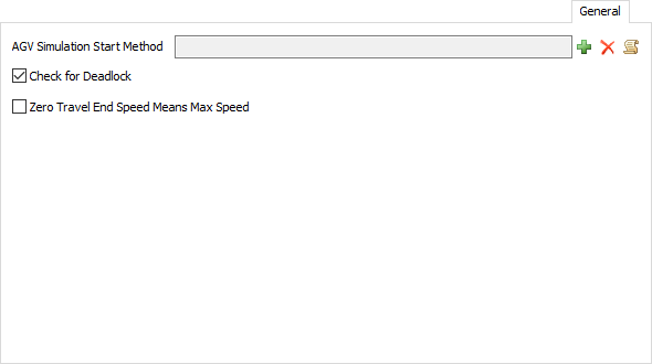
The General tab has the following properties:
You can get to the General page by right-clicking on a Path or Control Point and choosing AGV Network Properties.
AGV Simulation Start Method
A trigger that will fire for each AGV at the beginning of the model. Usually you will use this to fire the AGV's OnResourceAvailable, in order to start the AGV polling for work.
Check for Deadlock
If checked, the Control Point/Control Area allocation logic will continuously check for deadlock cycles. If it finds one, it will stop the model and notify you of the issue. Note that deadlock detection does require additional calculations and may slow your simulation down. You should hence turn it on while debugging, and once all deadlock issues are resolved, turn it back off.
Zero Travel End Speed Means Max Speed
If checked, AGV's will interpret travel tasks with end speed of 0 to mean: end at the AGV's max speed. This behavior is the default with other FlexSim travel mechanisms, such as standard travel networks that use network nodes. However, with AGVs this is not always the desired behavior, so it is an explicit setting that you define here.
Way Point Trigger Actions
The following sections explain the different way point trigger actions.
Redirect via Search
Redirect via Search will redirect the AGV by search through the Control Point Connections of the Control Point the AGV is arriving at.
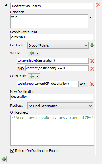
- Condition - The condition field specifies when you should execute this action. The default (true) means always execute the action. You can use the drop-down button on the right to help you fill in this field.
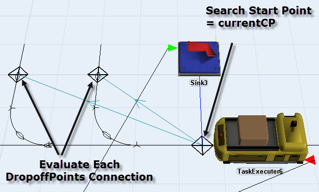
- Search Scope - Here you define the scope of the search. This includes a Search Start Point, which is the Control Point from which to start your search. The default, currentCP, is the Control Point where the AGV has arrived. Next, you define the set of Control Point Connections to search. The default, DropoffPoints, means that it will search all of currentCP's DropoffPoints connections, evaluating whether to dispatch to each of the resulting Control Points.
- Filter (WHERE) - The WHERE filter defines the
criteria for dispatching to a given Control Point in the search. The default is:
- The Control Point is available, i.e. it is not claimed by another AGV.
- The Control Point has nothing in it, i.e. there is not a flow item at that location waiting to be picked up.
- Prioritization (ORDER BY) - The ORDER BY parameter defines which Control Points are best to dispatch to if there are multiple matches. The default is to dispatch to the Control Point that is closest to currentCP.
- New Destination - The new destination that you want to dispatch to. This is usually just the matched Control Point itself, i.e. destination.
- Redirect Type - This parameter defines how you
want to redirect the AGV. The options are:
- Redirect as Final Destination - the AGV will finish the travel once arrive (as long as another Way Point doesn't redirect him again).
- Redirect and Wait - the AGV will travel to the destination and wait until it is redirected again
- Redirect and Continue - the AGV will travel to the destination and continue on to its original destination. If On-Arrival is chosen, the AGV will slow down to a stop at the intermediate destination before continuing. If On-Pre-Arrival is chosen, the AGV will just pass through the intermediate destination, not slowing down.
- On Redirect - A piece of code to execute when a valid AGV is found.
- Return On Destination Found - If checked, the Way Point trigger will discontinue execution if it finds an AGV to redirect to. The trigger will thus skip any subsequent logic. Sometimes you may daisy-chain multiple actions together, where you attempt to do one thing, and if you don't find anything to do, you try to do the next thing. If this is checked, then it will return when found, meaning you successfully found something to do for the AGV, and thus don't want to look for anything else.
Look For Work
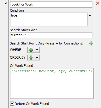
This action will search for work to do and take up work when found.
- Condition - Defines the condition by which to look for work. Same as the Redirect Via Search condition.
- Search Start Point / For Each - Defines the search scope. Similar to Redirect Via Search scope, except here it is searching the task sequence queues of the objects/Control Points in the search. The default only searches the task sequence queue of the AGV's current Control Point. You will often use the LookForWork action in conjunction with a FixedResource's Use Transport > Move Item Via AGV action. In such cases, task sequences will often be stored on the Control Points themselves, so the task queue search will be focused on Control Points' task queues.
- Filter (WHERE) - Defines criteria for taking up a given task sequence, i.e. loading/unloading a specific flow item. Similar to the Redirect Via Search filter, but here the focus of the filter is focused on a flow item, namely a task sequence's load/unload flow item.
- Prioritization (ORDER BY) - Defines prioritization. Again, like the Redirect Via Search prioritization, but here the focus is a flow item.
- Additional Parameters - Similar to Redirect Via Search additional parameters.
Redirect Via Direct Reference
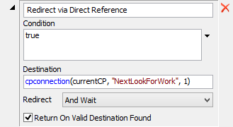
This action will redirect the AGV to another Control Point by a direct reference.
- Condition - Same as Redirect Via Search condition.
- Destination - The reference to the Control Point/object to redirect to.
- Additional Parameters - Similar to Redirect Via Search additional parameters.
Wait For Control Point Availability
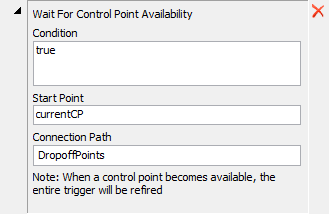
This action will wait for one of a set of Control Points to become available. When availability happens, all actions for the Way Point trigger will be refired. Usually you will place this action after a Redirect Via Search action, such that if nothing is found to redirect to, i.e. all Control Points are unavailable, you can wait for a Control Point to become available.
- Condition - Same as Redirect Via Search condition.
- Start Point / Connection Path - These fields define a set of Control Points to "listen to" for availability. The Start Point is a Control Point to start at, usually the AGV's current Control Point (currentCP). Connection Path defines the Control Point Connection(s) fanning out from the Start Point that enumerate the Control Points to listen to. The default is DropoffPoints. DropoffPoints would be used, for example, if you have a loaded AGV that needs to get into a spur to drop off its item, but currently all drop-off spurs are taken. So, you wait for a Control Point to become available, and you listen for availability on each of the drop-off points associated with the AGV's current Control Point. For Connection Path, you can define a single Control Point Connection, as in the default DropoffPoints, or you can define "chained" connections, such as "NextLookForWork > DropoffPoints". This would start at the Start Point, and fan out first to all of its NextLookForWork connections, and then for each of those it would enumerate all of the DropoffPoints connections.
Wait For Work
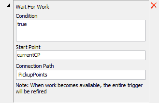
This action will wait for work to arrive at a defined set of Control Points. This should be used in conjunction with the Use Transport > Move Item Via AGV action. When that action is used, flow items will be placed in the Control Points for pick up. This Wait For Work action will listen for when items enter those Control Points, and then will refire all actions for the Way Point again. Usually you will add the Wait For Work after a Look For Work action, such that if no work is found, you can then wait for work to arrive.
Wait For Defined Delay Time
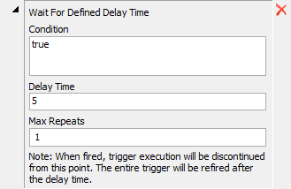
This action will wait for a defined delay time and then refire the Way Point trigger's actions again. Usually you put this at the start of a Way Point trigger. This can implement some delay associated with the real-life decision making process, i.e. if it takes the real-life system 5 seconds to process a dispatching decision, you first wait for 5 seconds, then fire the decision logic.