Introduction to Simulations
What is a Simulation?
In general, simulation models are digital imitations of a business system. In particular, a simulation can imitate the behavior of a business system over time. Using FlexSim, you can either build a simulation model that imitates your business system as it currently exists today or you can build a prototype of your future business system to predict its performance in the real world. (See Current State vs. Future State Models for more information about the pros and cons of building a current-state model or a future state-model.)
The purpose of a simulation model is to help you gain a deeper understanding of your business system and work on improving it holistically. Ideally, once you have built your simulation model, you will be able to experiment with different variables in order to better optimize your system. You could also use your simulation model to test how your business system responds to changing conditions.
However, you might find that even going through the work of gathering data to create your simulation model will give you some valuable insights in their own right. In the process of gathering data about your system, you will get a first-hand view of your system by making real observations in real time talking to real people. Those insights alone might help you identify ways to optimize your business system in a way you hadn't been able to see before.
What are Discrete Event Simulations?
A discrete event simulation has three main components:
- A model
- A clock
- An event list
A model generates events, which drive the simulation. An event is something that will change the model at a specific time. All events are placed on the event list, which sorts events chronologically. As the simulation runs, the clock time increases. When the clock time matches the next event time, that event updates the model and is removed from the list.
For example, the screen capture below shows a simple model running. You can see parts arrive from source, wait in the queue, and go through the processor before leaving the system. In this model, only one part can be processed at a time:
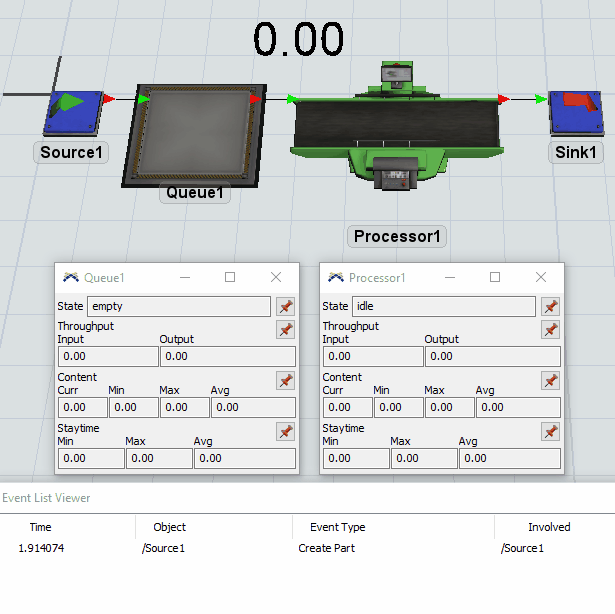
This example shows the model, the clock, and the event list. The model consists of the 3D objects. The clock is shown above the 3D objects. The event list is shown below the object statistic windows.
This example demonstrates the fundamentals of discrete event simulation. You can watch as the clock gets to an event, and then that event causes something to happen in the model. In addition, you can see that some events cause objects to create more events. For example, when the source creates a flowitem, it also creates an event to create another flowitem in the future. Finally, you can see that as the events occur, the statistics in the model are kept up to date.
One of the main advantages of discrete event simulation is that you can skip the time between events. This allows the simulation clock to move much faster than real time, even for complex models.
Continuous Values in Discrete Event Simulation
In the previous example, you can see values that change between events; flowitems travel smoothly across the processor, and the average content statistic changes frequently. This may seem to go against the nature of event-based simulation.
FlexSim simulates these kinds of values by recording key information with events. For example, when an item arrives on the processor, the processor records the arrival time. It calculates the time the part will be finished, and schedules an event at that time. This means that when the processor is drawn in the 3D view, it can use the current time and the item's arrival time to put the box in the correct position. The average content works in a similar manner. When the content changes, FlexSim can store enough information during that event to calculate the value between events, if that value is needed.
An Example of Using Simulation
Imagine you are building a simulation of an assembly line for car steering wheels and you are interested in determining whether your assembly line is running at its optimal efficiency level. In this simulation, a series of parts will arrive at a welding station. You might represent the welding station using a processor (a type of 3D object that simulates the time it takes to process a particular product) and an operator (the employee who needs to operate the welding machine).
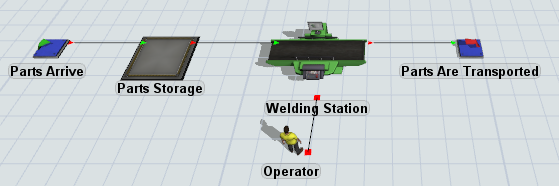
The arrival of the parts at the welding station would be an event. This event triggers the processor and operator to begin welding the parts together. Before the parts arrive, both the processor and operator might be idle, which is the specific state they are in before the parts arrive. After the parts arrive and the processor begins to weld the parts, the processor's state changes to processing (because it is processing the parts) and the operator's state changes to utilize (because the employee is being used). After the processor and operator finish welding the parts, the processor and operator return to their idle state.
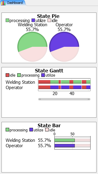
You can use then use these states to gather useful metrics about the efficiency of the assembly line. Perhaps you've decided that the key metrics you are interested is the amount of idle time compared to the amount of utilized time for both the operator and the processor. These metrics can help you determine whether your welding station and your employees were being under- or over-utilized:
- If your welding station and employees are being under- or over-utilized, it could mean that you haven't yet found the most efficient balance of resources in your business system to match customer demand.
- If your resources are over-utilized, you could have a bottleneck at that point in the assembly line.
You could then experiment by increasing the number of welding stations and employees. If your resources are under-utilized, you could analyze your business system to determine if there are bottlenecks earlier in the assembly line or if there are currently too many welding stations or employees.