Running Jobs
About Experiment Jobs
An Experiment Job defines a strategy for generating Scenarios, and for determining how many Replications of each Scenario to run. When you run a Job, the Experimenter will run the model once for each Replication of each Scenario, and record the results.
Please read Key Concepts About Experiments before reading the rest of this topic.
Opening the Experimenter
To open the Experimenter:
- On FlexSim's main menu, click the Statistics menu.
- Select Experimenter.
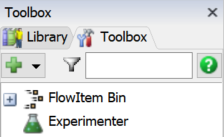
Once you've created an Experimenter, you can access it by double-clicking the Experimenter from the Toolbox.
Overview of the Experimenter User Interface
The Experimenter interface is a window that has multiple tabs. The following table explains the basic purpose of each tab:
| Tab | Purpose |
|---|---|
| Jobs | The Jobs is where you'll manage the list of Jobs for the Experimenter. You can use this tab to add, configure, reorder, and remove Jobs. |
| Run | You will use this tab to run a Job. This tab also shows the progress of each job as it runs in a chart. |
| Advanced | On this tab, you can specify general options that apply to all Jobs. These options deal with what data is collected, configuring and using remote CPUs, and setting Experiment triggers. Most users won't need to change anything on this tab. |
Experiment Jobs
The most commonly used Job type is the Experiment Job. The Experiment Job allows you to specify a set of Scenarios to run, as well as how many replications of each scenario to run.
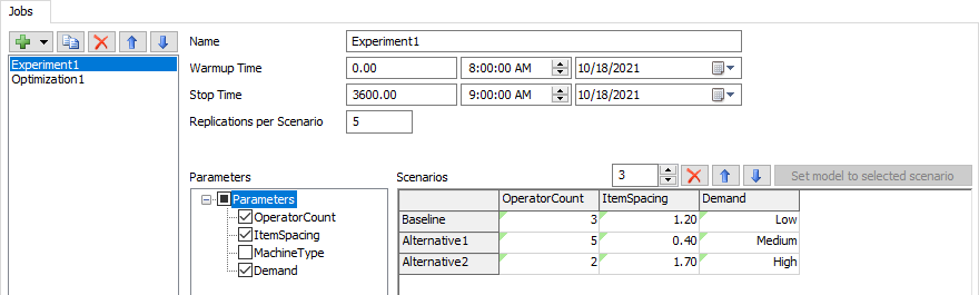
To configure the Experiment Job, you'll need to do the following:
- Set the Name of the Job. The name can be anything, but should be something that hints at the purpose of the Job.
- Set the Warmup Time. The value you specify will apply to all Scenarios.
- Set the Stop Time. The value you specify will apply to all Scenarios.
- Set the number of Replications. The Job will run this many Replications of each Scenario you define.
- Choose which Parameters to use. Adding a parameter adds a column to the Scenarios table. Note that all Parameters are included in each Scenario. If you don't use a particular Parameter, the Experiment Job will use the Parameter's current value for all Scenarios.
- Add Scenarios to run. Each Scenario is defined as a row of the table. You can set the value of each Parameter for each Scenario by editing the table. You can set the name of the Scenario by editing the row header.
Before running the job, also be sure that you have defined at least one Performance Measure. For more information, see the Performance Measures topic.
Running an Experiment Job
To run your experiment, you will use the Run tab in the Experimenter, as shown in the following image. Then use the Job field to select your Experiment Job.
The following sections will explain the various stages of running an experiment.
Before Running an Experiment Job
Before running an Experiment Job, you'll be able to see the status of any Scenarios your Job defines:
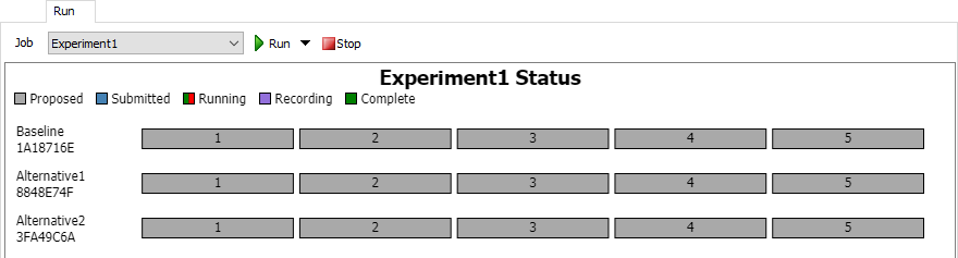
Below the chart's title and legend, there is one box per Task generated by the Job. These boxes are organized by Scenario, and display the Replication number for that Task. If you haven't run the Job before, then all Tasks will be marked as "Proposed", meaning there is no data in the Results Database File connected with those Tasks. The chart also shows the name and hash of each Scenario.
You can hover over any Scenario on the chart, and a magnifying glass icon 🔍 will appear. You can click on that icon to see a popup with additional information about each Scenario.
Running an Experiment Job
Click the Run button to run the Job. At this point, the Experiment Job submits all Tasks to the Experimenter. The Experimenter checks for any Tasks that have already been completed, and ignores those Tasks. All other tasks are added to the Results Database File at that point. On the chart, you'll be able to see those tasks change to "Submitted". Once the Task begins, you'll see a progress bar for that Task. The progress bar shows how much model time has elapsed, compared to the Stop Time as a percentage. When the model reaches the stop time, the task will be marked as "Recording". During this phase, the results are calculated and stored in the database file. Once all the results have been recorded, the Task is marked as "Complete":
After Running an Experiment Job
When a Job has finsihed running, click the View Results button to open a separate window with the results. The Experiment Results window has six tabs:
| Tab | Purpose |
|---|---|
| Performance Measures | This tab will display the results of the experiment for each performance measure that you defined. Use the menu to select the specific performance measure you want to display. |
| Dashboard Statistics | This tab will display dashboard charts from any of the scenarios and replications you are interested in exploring. Be aware that you need to first add the charts you are interested in to your Dashboard in your simulation model before you can use this tab. |
| Statistics Tables | This tab displays the data for each Output Table (Statistics Collector or Calculated Table). The data from all Tasks is included in this table, sorted by Scenario and Replication. |
| Result Tables | This tab displays each Result Table. A Result Table is a configurable table that shows Scenarios or Replications as rows, with Parameters and Performance Measures as columns. |
| Console Output | Use this tab to check that there weren't any errors in your simulation models when you ran the experiment. This tab will allow you to check the console output for each replication for any console error messages. Make sure you don't skip looking at this step. |
| State Files | If you have saved state files, those files will be accessible here. |
The following image shows an example of the results:
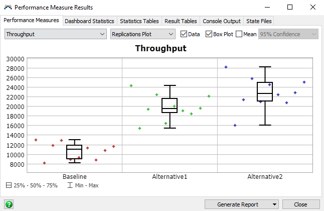
You can see that both the Alternative1 and Alternative2 Scenarios had a higher Throughput than the Baseline Scenario.
Re-Running Replications or Scenarios
There may be rare cases where you'd like to re-run a particular Scenario or Replication, without re-running the whole Experiment. From the Run tab on the Experimenter, you can hover over any completed Scenario or Replication, and a remove button ❌ will appear. If you remove results, then run the Job again, those Tasks will be run again.
These cases are rare. There are not very many reasons to re-run a model. One particular case might be that a bug occurred in a particular Scenario or Replication, and you'd like to fix that bug, then re-run the associated Tasks. You must be able to guarantee that the change you made would not affect the results of any other Task, and that can be difficult to prove. It is usually better to re-run the entire Job, so that all results are generated by the same model.
Optimization Jobs
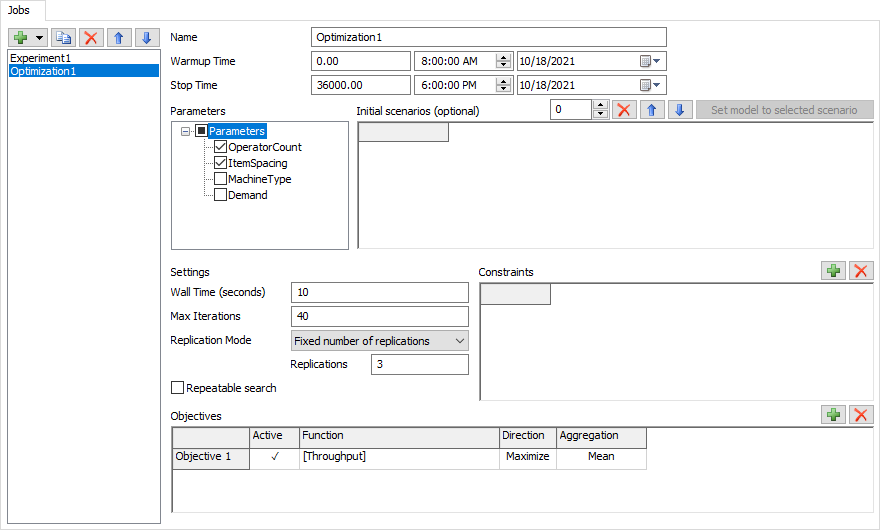
An Optimization Job is useful when you are trying to find the Parameter values that produce the best behavior in your model. Unlike an Experiment Job, you don't need to specify Scenarios. Instead, you simply specify two things: which Parameters can be varied, and an Objective. An Objective is a scoring function, as well as an option to either maximize or minimize that score.
When you run an Optimization Job, the will start by generating random Scenarios and running Replications of those Scenarios. As Tasks complete, the Optimization Job will analyze the results and generate new Scenarios that perform better. Given enough time, an Optimization Job can often find a Scenario that performs very well.
You'll use the following steps to configure an Optimization Job:
- Set the Name of the Job. The name can be anything, but is most helpful if it hints at the purpose of the Job.
- Set the Warmup Time. The value you specify will apply to all Scenarios.
- Set the Stop Time. The value you specify will apply to all Scenarios.
- Choose which Parameters to use. The Optimization Job will only adjust the values of the Parameters you specify.
- Optionally, specify any Initial Scenarios. The Optimization Job will evaluate these Scenarios early in the search. This is a way for you to provide a good starting point for the search, which can save time.
- Optionally, specify any Constraints. Constraints are described in a later section.
- Set the Wall Time and Max Iterations. These both control when the Optimization Job will stop. The Wall Time is the approximate number of seconds the Optimization Job will run for; if it exceeds that time, it wil stop. To stop the Optimization after 10 minutes, enter 600 in this field. The Max Iterations specifies the maximum number of Scenarios to evaluate. The Optimization Job will stop after evaluating this number of Scenarios.
- Specify the Replication Mode and the number of Replications. The most common setting is to run a fixed number of Replications.
- Define one or more Objectives. The next section discusses Objectives in more detail.
Adding Objectives
You need to define what success looks like so that the Optimizer can determine which Scenario best meet that definition. You'll do this by adding your specific goals to the Objectives table.
An Objective contains a simple function. For example, you may be interested
in maximizing the throughput of your system. If you had a Performance Measure
called Throughput, your expression would look like this: [Throughput].
The function can include references to any Parameter or Performance Measure.
Those names should be in sqare brackets.
The function can also include basic math operations, such: as [Throughput] * 300.
Note that each objective has an Active field. Only the active objectives are included in an optimization. If more than one objective is active, the Optimization Job will perform a multi-objective search. If only one objective is active, the Optimization Job will perform a single-objective search. You need at least one active objective to run the Optimization Job.
Adding Constraints
Constraints are a way of specifying additional conditions that a given model must maintain. The Optimization Job will only mark a configuration as optimal if it is feasible within the constraints you've defined.
Constraints are very different from objectives. An objective is a scoring function; the Optimization Job is trying to find parameters that improve the scores. A constraint is a pass-fail test. The Optimization Job will evaluate whether a given solution passes all the tests. If it does, then the solution is considered feasible. If the solution fails any of the tests, the Optimization Job considers that solution as infeasible. The Optimization Job will try to find the best feasible solution.
Constraints are expressions that involve a ≤ or a ≥ comparison. Here are some example constraint equations:
[OnTimeJobsPercent] >= 0.80[ReworkParts] <= 10[Utilization] >= 0.75[PackTeamSize + ShipTeamSize] <= 30
In some cases, a constraint is there to enforce performance standards while optimizing. The Optimization Job is very focused, and without a constraint, may give you an unhelpful answer. For example, if you have an objective to maximize throughput, the Optimization Job might increase the number of employees to an absurdly high number. Throughput is fantastic, but maybe utilization is unacceptably low. To avoid this issue, you could add a constraint, so that utilization must be kept at or above a certain threshold. Constraints that involve Performance Measures are evaluated after the replication has been run.
In other cases, a constraint is there to enforce rules between multiple Parameters. For example, the Optimization Job might be allowed to increase the number of people on various teams. However, you might want to keep the total number of people below 30. So you could add a constraint that specifies the sum of several Parameters is less than some number. A constraint that only involves constants or Parameter values can be evaluated without actually running the replication. They just help the Optimization Job suggest valid Scenarios.
Running an Optimization Job
To run an Optimization Job, you will use the Run tab of the Experimenter. Select the correct Job, and press the Run button:
The Optimization Job Status Chart
The Optimization Job has different status chart than the Experiment Job. The chart shows each Scenario as a point on a scatter plot. By default, the X axis shows the iteration number, and the Y axis shows the first objective. You can configure either axis to show values related to the Scenario, including the Parameters, Performance Measures, and Objective values.
You can optionally choose to set the color of each point based on one of the Objective values. This can help you explore the relationships between Parameters, Peformance Measures, and Objectives.
The best Scenarios are marked with a gold star ★. If you have a single Objective, the Scenario with the star is the best the Optimization Job found before it was stopped. If you have multiple Objectives, there will be a star on each Scenario that is on the trade-off curve. If a Scenario is in the trade-off curve, it means that no Scenario was found that can improve any Objective without worsening another Objective.
You can also select Scenarios by clicking on a point. A ring will appear around the Scenario. The color of the ring is consistent so you can select a point, then change the X, Y, and Color axis, and still see the selected Scenario.
Viewing the Results
Because all jobs share the Results Database File, you can click the View Results button in the Experimenter to open the Performance Measure Results window. This window shows all results, reguardless of which Job generated those results.
Range-Based Jobs
A Range-Based Job is very similar to an Experiment Job. They both allow you to define a specific set of Scenarios, as well as the number of replications to run for each Scenario. They differ in how you specify scenarios. An Experiment Job requires you to specify the value of all involved parameters for every scenario. A Range-Based Job, on the other hand, allows you to specify a set of values for each parameter. When you run the Range-Based Job, it generates one Scenario for every combination of parameter values.
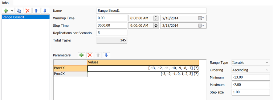
The job in the preceding image would generate 49 Scenarios. The job also specifies that each Scenario will run for five Replications, for a total of 245 tasks.
To use this job, you can add model parameters to the Parameters table in the job's interface. Any parameters you don't specify are assumed to stay at their current values.
The job generates scenarios using the order of the parameters and values defined in the table. The job in the preceding image would generate scenarios in the following order:
| Proc1X | Proc2X |
|---|---|
| -13 | -3 |
| -13 | -2 |
| ... | ... |
| -13 | 2 |
| -13 | 3 |
| -12 | -3 |
| -12 | -2 |
| ... | ... |
For each parameter, you can specify a range. The range is the set of values for that parameter. For numeric types, you can specify that range in terms of a minimum, a maximum, and step size. For any parameter, including Expression and Sequence parameters, you can define the set of values explicitly. To do so, change the Range Type from Iterable to Specific Values.
Running Range-Based Jobs
When you run a Range-Based Job, you'll see a chart with two main sections: a progress bar, showing the progress of the job, and a grid of squares, where each square represents a Scenario.
The chart arranges the Scenario squares into blocks, where all the Scenarios in that block have some parameter values in common. The common parameter values are used to create the title of the block.
You can click on any scenario to see see more information about it in the footer of the chart. From there, you can click the 🔍 button to see the parameters for that scenario, or rename the scenario. If you hover over a replication box, you can click the 🧪 button to apply that replication to the model. You can also click on the ❌ button to delete the results from the scenario, or from one of its replications.
Viewing the Results
Because all jobs share the Results Database File, you can click the View Results button in the Experimenter to open the Performance Measure Results window. This window shows all results, reguardless of which Job generated those results.
Running Jobs on the Cloud
The Experimenter can use remote computers to run replications of a model. Normally, when you run a job, the Experimenter launches many instances of FlexSim on the same computer. It then communicates with those instances to run replications of the model. When using remote computers, FlexSim sends HTTP requests to servers at IP addresses you specify. Each of those servers launches FlexSim instances, and the Experimenter then communicates over the network or internet to with those instances.
A remote computer must meet the following requirements:
- The FlexSim Webserver must be running on the remote computer.
- The exact same version of FlexSim must be installed on the remote computer.
- The IPv4 address of the remote computer's webserver must be specified in the Global Preferences on the local computer.
- The remote computer does not need to be licensed.
Once the remote computers are configured, you simply need to check the Use distributed CPUs box on the Advanced tab of the Experimenter.
Querying Experiment Tables
You can use SQL to query data from the Results Database File.
| Table Type | Example Query |
|---|---|
| Result Tables. You can add, edit, and remove Result Tables on the Result Tables tab of the Performance Measure Results window. | |
| Statistics Tables. These are the tables found on the Statistics Table tab of the Performance Measure Results window. The include all Statistics Collectors, Calculated Tables, People Statistics Tables, and Chart Templates. | |
| Legacy Experiment Tables. For backwards compatibility, you can query the Scenarios table, as well as the PerformanceMeasures table. Summary tables replace and improve both of these tables. | |
You can run these queries using FlexScript or a Calculated Table. If you are familiar with SQL queries, you can use these tools to explore the result data further.