Task 4.2 - Optimizer
Task Overview
In addition to using the Experimenter to explicitly define scenarios, you can use the Optimizer. The Optimizer will automatically create scenarios and then test those scenarios, trying to find a scenario that best meets an objective.
Step 1 Designing the Optimization
-
Go to the Optimizer Design tab in the Experimenter window. You will see that the two variables created earlier are present; this is because the Experimenter and Optimizer share variables.
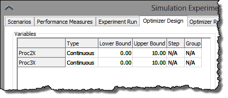
However, the Optimizer needs additional information about those variables. Specifically, you must specify:
- Type - The type of a variable dictates what kinds of values are possible for a given variable. Continuous variables can have any value between the upper and lower bound.
- Lower Bound - The lower bound specifies the lowest possible value the Optimizer can set for the variable.
- Upper Bound - The upper bound specifies the highest possible value the Optimizer can set for the variable.
- Step - For Discrete and Design variables, the step specifies the distance between possible values, starting from the lower bound.
- Group - For permutation variables, the group specfies which set of permutation variables this particular variable belongs to.
-
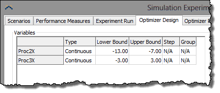
For this optimization, we want to allow the processors to move three meters to either side. Since we are not limited to specific positions within that range, both position variables are Continuous. However, we need to set the lower and upper bounds of each variable. To edit values in the table, double-click on the cell of interest and enter in the new value. Enter in the values shown below:
-
The final design step is to set the objective function. The objective function is present, but blank. Edit its name to be Revenue. Then click on the function field. A
 button will
appear on the right side. Click on this button to bring up a list of all variables
and performance measures. The objective function is a value derived from any or
all of these values. Select Throughput; this will add
that perfomance measure to the objective function, and put the cursor right and
the end. Add the text
button will
appear on the right side. Click on this button to bring up a list of all variables
and performance measures. The objective function is a value derived from any or
all of these values. Select Throughput; this will add
that perfomance measure to the objective function, and put the cursor right and
the end. Add the text * 500so that Revenue is equal toThroughput * 500. Leave the direction on Maximize, because we want to maximize Revenue. Since we only have one objective, the search mode can remain on Single.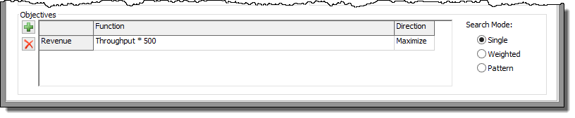
Step 2 Running the Optimization
-
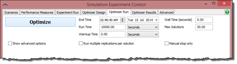
Go to the Optimizer Run tab in the Experimenter window. Then:
- Set the Run Time to
10000. This is how long the Optimizer will run each model configuration (called a solution) to evaluate it. - Set the Wall Time to
0. This usually means how long the Optimizer is allowed to run in real time. The value 0 means it has no time limit. - Set Max Solutions to
50. This means the Optimizer will try no more than 50 different solutions to find the optimal solution. - Click the Optimize button.
- Set the Run Time to
-
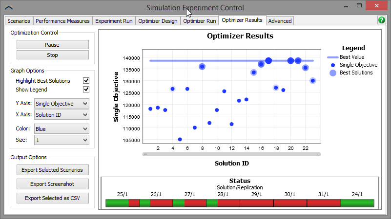
The Experimenter window will automatically switch to the Optimizer Results tab. The Optimizer then begins running through the following loop:
- Determine values for Proc2X and Proc3X.
- Run a model with those values for 10000 seconds.
- Evaluate the performance measures.
- Calculate the objective function.
- Rank this solution.
- Use the information from this solution to create a new solution - new values for Proc2X and Proc3X.
- Repeat from Step 2.
-
Because the Optimizer shares the multi-threaded capability of the Experimenter, it can evaluate multiple solutions at the same time. As the optimization progresses, the Optimizer Results graph will update and show the Optimizer's progress.
-
Once the Optimizer evaluates 50 solutions, a message will appear stating why the Optimizer stopped. In this case, it will say that the Optimizer reached the maximum number of solutions. If something went wrong, the message will contain information about the error.
Step 3 Analyzing the Results
When the optimization is finished, the Optimizer Results chart should look something like this:
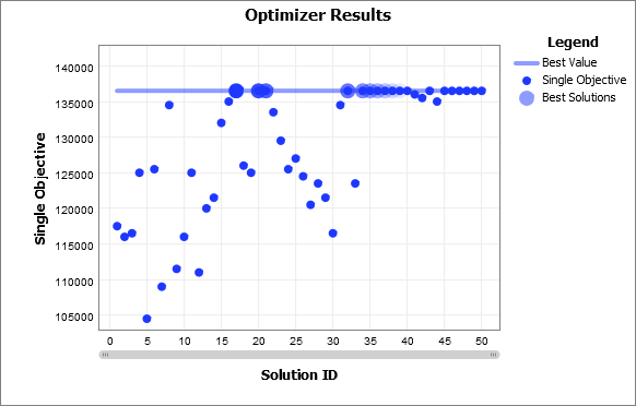
The Y Axis is called "Single Objective". For this example, it is synonymous with Revenue. The best solutions are highlighted. The circles with a lighter border around them represent better solutions. For a single objective, the top 10 solutions are marked this way.
As the optimization progressed, the Optimizer got better and better at creating good solutions, so that the last 15 solutions were all very good. This is called convergence, and it is one way to tell if an optimization is finished; if the objective value has not improved for a while, it may be that it will not improve with further searching, and the current best solution should be used.
Answering the Original Question
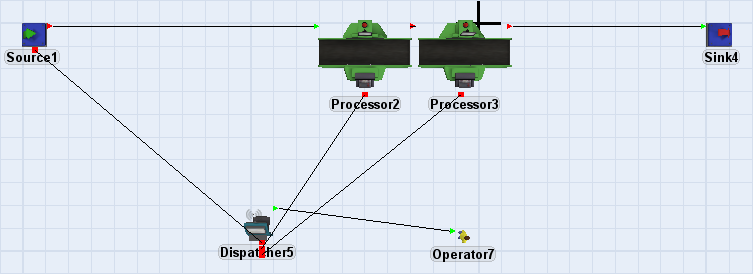
The goal of this optimization was to figure out where to put the two processors. We can now very easily find the answer to this question.
-
Hover over the best solution (the largest blue circle) on the chart; a small popup will appear.
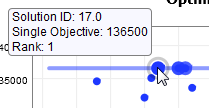
-
Click on this solution to select it. Now, in the Graph Options panel, change the Y Axis to Proc3X, and the X Axis to Proc2X.
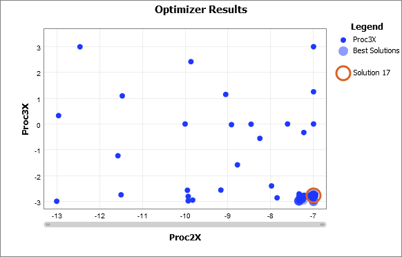
-
The best solution (and all the other best solutions) is found where Proc2X is greatest, and where Proc3X is least. Remember that all top 10 solutions produced the same results; in this case, having the two processors right next to each other is the best configuration for this model.
Setting the Model to the Best Solution
It can be very useful to set the model to match the best solution. To do this:
-
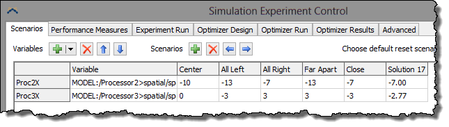
Click the Export Scenarios button. This takes all the selected solutions and creates Experimenter scenarios for them. Go back to the Scenarios tab on the Experimenter window to view the new solution.
-
Now, from the Choose default reset sceanrio drop-down on the far right, select the new scenario. Then reset the model to apply those values to the 3D model.
Conclusion
At this point, you've learned how to use the Optimizer.