SQL Queries
Overview and Key Concepts
FlexSim provides a flexible method for querying, filtering and prioritizing data in a model using the SQL language. Using SQL queries, users can do standard SQL-like tasks, such as searching one or more tables in FlexSim to find data that matches criteria as well as prioritizing that data. Instead of using FlexScript code to manually loop through and sort table data, you can write a single SQL query using the Table.query() command to do all the work for you.
For example, let's say you have a global table in your model that looks like the following:
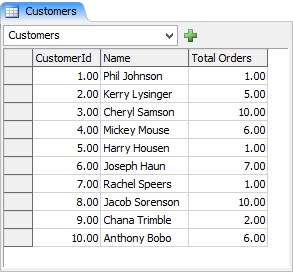
And let's say you want to search that table to find the name and id of the customer with the most total orders. The manual method for doing this in FlexScript would look like the following:
		Table customers = Table("Customers");
		int bestRow = 0;
		int highestTotalOrders = 0;
		for (int i = 1; i <= customers.numRows; i++) {
			int totalOrders = customers[i][3];
			if (totalOrders > highestTotalOrders) {
				bestRow = i;
				highestTotalOrders = totalOrders;
			}
		}
		int bestCustomerId = result[bestRow]["CustomerId"];
		string bestCustomerName = result[bestRow]["Name"];
Alternatively, using SQL and FlexSim's Table.query() command, you can do it much more simply, as follows:
		Table result = Table.query("SELECT CustomerId, Name FROM Customers \
			ORDER BY [Total Orders] DESC LIMIT 1");
		int bestCustomerId = result[1]["CustomerId"];
		string bestCustomerName = result[1]["Name"];
This is a pretty simple example. More complex tasks such as sorting multiple results or searching multiple tables would be much more complex to perform manually in FlexScript, whereas doing those complex searches using SQL is relatively easy once you understand the rules of SQL and how to write SQL queries.
FlexSim's SQL functionality also includes advanced querying techniques. These allow you to do searches on data in the model that are not structured like standard tables. You can search flow items, task sequences, resources, really any data in a model that can be conceptualized into lists.
Example
The following sections will guide you step-by-step through all the major concepts related to SQL queries.
Your First SQL Query
In FlexSim, SQL queries are done using the Table.query() method:
static Table Table.query(str queryStr[, ...])
Often you will use the Table.query() command to search a single table. Take the following example global table.
Let's say you want to find all customers who have made more than 5 orders, sorted alphabetically by their name. To do that, you'd use the following command:
		Table result = Table.query("SELECT * FROM Customers \
			WHERE [Total Orders] > 5 \
			ORDER BY Name ASC");
- The
SELECTstatement tells the query what columns you want to pull out into your query result. By usingSELECT *we are telling the query to put all the columns from the source table into the query result. Alternatively, if we were to useSELECT CustomerId, Namethen that would put just the CustomerId and Name columns into the query result. - The
FROMstatement defines the table that is to be queried. Often this will be just one table, but it may be multiple comma-separated tables, which effects a join operation, discussed later. Here we defineFROM Customers. This causes the SQL parser to search the global table in the model named Customers. - The
WHEREstatement defines a filter by which entries in the table are to be matched. The expressionWHERE [Total Orders] > 5means that I only want rows whose value in the Total Orders column is greater than 5. In aWHEREstatement you can use math operators to define expressions, like+,-,*,/and logical operators like==,!=(also<>),<,<=,>,>=,AND, andOR. - The
[ ]syntax is an SQL delimiter that allows you to define column names with spaces in them. If I had named the column TotalOrders instead of Total Orders, I could have just putTotalOrdersfor the column name in the query instead of[Total Orders]. - The
ORDER BYstatement defines how the result should be sorted. Here we sort by the Name column, which is a text column and thus will be sorted alphabetically. You can optionally putASCorDESCto define if you want it sorted in ascending order or descending order. Default is ascending. You can also have multiple comma-separated expressions defining the sort. The additional expressions will define how to order things when there is a tie. For example, the expressionORDER BY [Total Orders] DESC, Name ASCwould first order descending by the number of total orders, and then for any ties (Cheryl Samson and Jacob Sorenson both have 10 total orders) it would sort alphabetically by name. - The
\escape character lets you extend a quoted string across multiple lines by using the\at the end of a line within a string. Often with SQL queries, the query is too long to reasonably fit within a single-line quoted string. Also, using multiple lines with indentation can make the query more readable. - A
LIMITstatement, although not used in this example, can be added at the end of the query. This will limit the number of matches. If you only want the best 3 matches, addLIMIT 3to the end of the query.
Getting Data Out of the Query
Now that you've done your query, the result is stored in a read-only in-memory instance of a Table. To copy the entire result to something like a global table, or a table on a node in the tree, you can use Table.cloneTo(). This will copy a query result to a table or bundle node. For this example we can create a global table named QueryDump, and then copy the result to that table.
		Table result = Table.query("SELECT * FROM Customers \
			WHERE [Total Orders] > 5 \
			ORDER BY Name ASC";
		result.cloneTo(Table("QueryDump"));
Dumping the above query to the global QueryDump table yields the following results:
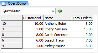
Table Selection
The SQL language is designed to generate a result table from a set of input tables.
In the example above, we used "SELECT * FROM Customers". The
FROM tells the parser to look in global tables for a table named Customers and
search that table. In FlexSim, you can use any of the following tables in a from statement:
- Global Tables
- Global Lists
- Global StatisticsCollectors
- Global CalculatedTables
In addition, there are a few tables that deal with experiment or optimizer data. The following list enumerates and describes the tables that belong with experimenter data:
- Experiment.Scenarios - This table has a column for the scenario number and a column for each experiment variable. Each row represents the configuration of the given scenario for that row. This table reads the experimenter data, and is not affected by the optimizer.
- Experiment.PerformanceMeasures - This table has a column for both the scenario number and replication number, and an additional column for each peformance measure. Each row shows the value of all performance measures for the scenario and replication number. If you have run an optimization, this table will show the results from the optimization.
- Experiment.MyStatisticsCollector - This table is the result of concatenating the data from MyStatisticsCollector (or any statistics collector in the model) for all scenarios and replications, and adding two columns for scenario number and replication. This makes it possible analyze the data from a statistics collector across all replications and scenarios, in a single query.
Alternatively, you can explicitly define the tables for search. This is
done by using a special '$' identifier in the query and by passing additional
parameters into the Table.query() command. For example, I could have defined the exact same
query as above, but instead defined the customers table explicitly as follows:
		Table.query("SELECT * FROM $1 \
			WHERE [Total Orders] > 5 \
			ORDER BY Name ASC",
		current.labels["Customers"]));
Notice that instead of using the table "Customers" I now define the table as
$1. What this means is that the table I want searched is the table I pass in as
the first additional parameter of the Table.query() command. $2 would
correspond to the table passed into the second additional parameter of the command, and so
on. Tables passed as additional parameters can have either regular tree table data or bundle
data. However, they should not be an in-memory result Table, like the result of another call
to Table.query(). In other words, they must be stored on a node in FlexSim's tree in order
for FlexSim to process them properly.
By using this table specification method you are no longer bound to using global tables. For example, if the customers table happened to be on a label instead of a global table, the query is still pretty simple:
		Table.query("SELECT * FROM $1 \
			WHERE [Total Orders] > 5 \
			ORDER BY Name ASC",
		current.labels["Customers"]));
FlexSim's SQL parser also allows you to simpify the SQL a bit for this single-table
search scenario. The SQL standard requires a SELECT and FROM
statement, but FlexSim's SQL parser isn't that picky. If you only pass one parameter as the
table, it will automatically assume that you want to search the table you passed in. Thus
you can leave out the SELECT and FROM statements. Leaving them out is essentially the same
as using the statement SELECT * FROM $1.
Table.query("WHERE [Total Orders] > 5 ORDER BY Name ASC", current.labels["Customers"]);
Additional Result Analysis Methods
While using Table.cloneTo() is often useful when you're setting up a model
or when you're testing various queries, cloning an entire table/bundle with data is
non-trivial and requires memory space and CPU time for creating the table. Alternatively,
you can simply use the methods and properties provided by the
Table
class to process the result directly.
		Table result = Table.query("SELECT * FROM Customers \
			WHERE [Total Orders] > 5 \
			ORDER BY Name ASC");
		result.cloneTo(Table("QueryDump"));
		for (int i = 1; i <= result.numRows; i++) {
			string name = result[i]["Name"];
			...
		}
Joins
You can also use FlexSim's SQL parser to query relationships between multiple tables. To demonstrate this, we'll do another example using the Customers table and an additional Orders Table.
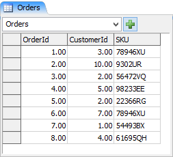
In this example we want to find information associated with customers who ordered SKU 78946XU. For each order of SKU 78946XU we want to know the customer's name, the CustomerId, and the OrderId. Below is the query:
		Table result = Table.query("SELECT * FROM Customers, Orders \
			WHERE \
			SKU = '78946XU' \
			AND Customers.CustomerId = Orders.CustomerId");
Things to note:
- Here we use the statement
FROM Customers, Orders. In SQL this is called an inner join. The SQL evaluator compares every row in the Customers table with every row in the Orders table to see which row-to-row pairings match theWHEREfilter. - The filter we define is
WHERE SKU = '78946XU' AND
			Customers.CustomerId = Orders.CustomerId
. We only want to match the rows in the Orders table that have the SKU value '78946XU'. Secondly, for those rows that do match the SKU, we only want to match them with rows in the Customers table that correspond with the same CustomerId in the matched row of the Orders table. - Notice that for the SKU rule we just say
SKU = '78946XU'. For SKU, since the Orders table is the only table with an SKU column, the SQL evaluator will automatically recognize that the SKU column is associated with the Orders table. We could explicitly define the table and column withOrders.SKU, and sometimes that is preferable in order to make the query more readable/comprehensible. However, if you leave it out the evaluator will happily figure out the association on its own. - The CustomerId rule, on the other hand, uses the . (dot) syntax to explicitly define table and column. This is because both the Orders table and the Customers table have columns named CustomerId, and we want to explicitly compare the CustomerId column in Customers with the CustomerId column in Orders. So we use the dot syntax to define table and column.
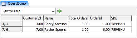
The result of the result.cloneTo(Table("QueryDump")) for this query:
For explicitly defined tables (labels for example) you'd use a query like:
		Table result = Table.query("SELECT * FROM $1 AS Customers, $2 AS Orders \
			WHERE \
			SKU = '78946XU' \
			AND Customers.CustomerId = Orders.CustomerId",
		current.labels["Customers"],
		current.labels["Orders"]);
Aliases
In the previous example we use the AS construct to create an alias for our
table. You can create aliases for both tables and column references. This can increase
readability of the query especially if you are using the $ syntax. For table
aliases you do not technically need the AS qualifier. Both of the following are
valid:
SELECT * FROM $1 AS Customers, $2 AS Orders
SELECT * FROM $1 AS Customers, $2 AS Orders
Once an alias is defined you should use that alias instead of the table name in other references in the query.
Below are several examples of defining column aliases.
SELECT Customers.CustomerId AS ID, Customers.Name AS Name
WHERE ID > 5 AND ID < 10
Advanced Query Techniques
Often there are decision-making problems in a simulation that lend themselves well to using SQL-like constructs, such as searching, filtering and prioritizing. However, since a simulation is an inherently dynamic system, data in the simulation is often not structured in the standard way that a database is structured. FlexSim's advanced SQL querying functionality aims to bridge this gap, allowing modelers to use SQL's flexibility and expressiveness in dynamically querying the state of a model.
Let's take an example where you have flow items that queue at various locations in the model. It is quite often the case that modeling logic will try to search for a "best" flow item, and determining which flow item is the best may involve complex rules. It might assign certain eligibility criteria for each flow item. It could also weigh various things like the distance from some source to the location of the flow item, the time that the flow item has been waiting in queue, an assigned priority for the flow item,etc. For these types of problems, the SQL language is quite expressive and makes the problem relatively easy. So what if you could represent all of the candidate flowitems as a kind of quasi-database table, and then use SQL to search, filter, and prioritize entries in that table?
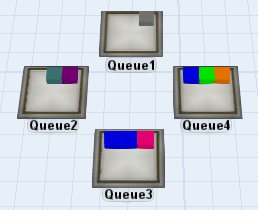
Here there are four queues, each with a set of flow items in it. Imagine each of those flow items has various labels defining data on that flow item. A table of flow items representing all of that data might look something like the following:
| Item | Location | DistFromMe | Priority | Step | ItemType | Time Waiting |
|---|---|---|---|---|---|---|
| GrayBox | Queue1 | 9.85 | 3 | 5 | 6 | 5.4 |
| PurpleBox | Queue2 | 8.5 | 2 | 2 | 8 | 8.1 |
| TealBox | Queue2 | 8.5 | 8 | 12 | 5 | 7.2 |
| OrangeBox | Queue4 | 12.5 | 4 | 1 | 4 | 1.2 |
| GreenBox | Queue4 | 12.5 | 3 | 5 | 2 | 4 |
| BlueBox | Queue4 | 12.5 | 6 | 6 | 3 | 22.5 |
| PinkBox | Queue3 | 7.5 | 3 | 9 | 7 | 12.8 |
| BlueBox | Queue3 | 7.5 | 6 | 10 | 3 | 3.4 |
| BlueBox | Queue3 | 7.5 | 4 | 7 | 3 | 7.1 |
If we could represent the model structure in these quasi-table terms, we could use SQL to do complex filtering and prioritizing based on those tables.
First, let's start simple. We'll just search one queue of flow items, Queue4, and we'll only look at the Step value, which, we'll say is stored on the items' "Step" label. We want to find the flow items with a step value greater than 3. The more simplified table would look like:
| Item | Step |
|---|---|
| OrangeBox | 1 |
| GreenBox | 5 |
| BlueBox | 6 |
Here's the command:
		Table result = Table.query("SELECT $2 AS Item, $3 AS Step \
			FROM $1 Queue \
			WHERE Step > 3",
		/*$1*/node("Queue4", model()),
		/*$2*/$iter(1),
		/*$3*/getlabel($iter(1), "Step"));
The results of result.cloneTo() on this would be:
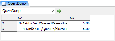
Here we introduce two new concepts: 1. object references as tables, and 2. individual
column values being defined by the $ syntax, instead of just tables.
Object References as Tables
The query table is defined with:
FROM $1 Queue
And we bind the $1 reference with:
node("Queue4", model())
Here instead of referencing an actual table, we reference an object in the model. In doing this, we're associating each row of our "virtual table" with a sub-node of the object we reference, or in other words, a flow item in the queue. So the first row in the table is associated with the first flow item inside the queue, the second row with the second flow item, and so on.
$'s as Table Values and $iter()
The select statement looks like this:
SELECT $2 AS Item, $3 AS Step
And we bind $2 with:
getlabel($iter(1), "Step")
And $3 with:
getlabel($iter(1), "Step")
Again here's the "virtual table" we are searching, based on each flow item in Queue4 and its Step label.
| Item | Step |
|---|---|
| OrangeBox | 1 |
| GreenBox | 5 |
| BlueBox | 6 |
We use the $iter() command to determine the values of the table cells by
traversing the content of Queue4. $iter() returns the iteration on a given
table. $iter(1) is the iteration on $1. Since $1 is
Queue4, $iter(1) is going to be the iteration on Queue4 associated with a given
row in the table, or in other words, one of the flow item sub-nodes of Queue4.
When the evaluator needs to get the value of a certain row in the table, it sets
$iter(1) to the flow item sub-node of Queue4 associated with that table row,
and then re-evaluates the expression. So when it's on the GreenBox row in the table (row 2)
and needs to get the Step value for that row, it sets $iter(1) to
rank(Queue4, 2), and evaluates $3. $3 then
essentially returns getlabel(rank(Queue4, 2), "Step"). That value is then used
as the value of the table cell.
Creating a Table for All Flow Items
Now that we've done a query on a single queue, let's extend the query to search all queues. Let's assume the queues are all connected to the output ports of an upstream queue.
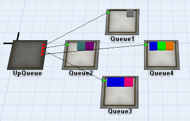
Now let's write the query.
		Table result = Table.query("SELECT $3 AS Item, $4 AS Step \
			FROM $1x$2 AS Items \
			WHERE Step > 3",
		/*$1*/nrop(node("UpQueue", model())),
		/*$2*/outobject(node("UpQueue", model()), $iter(1)),
		/*$3*/$iter(2),
		/*$4*/getlabel($iter(2), "Step"));
The results of result.cloneTo() on this query are as follows:
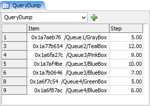
Note that we've shifted our column references down. The Item reference is now
$3 and the Step label reference is $4. Also notice that we've
"flattened" a two-dimensional model structure into a single virtual table by using the
special table identifier $1x$2. The first dimension is the output ports of
UpQueue, and the second dimension is the sub-node tree of each of the Queues connected to
the output ports of UpQueue.
Numbers as Tables
For $1 we return nrop(node("UpQueue", model()) Unlike
previously where we assigned $1 to a Queue object itself, now we define
$1 as a straight number, namely the number of output ports of UpQueue.
Subsequently, the iteration on $1 ($iter(1)) will also be a number.
"Flattening" Model Structures
When the SQL parser sees the special $1x$2 table reference, it will "build"
the table by evaluating $1 and then iterating on $1, evaluating
$2 for each iteration. In this example, it evaluates $1 which
returns 3, the number of output ports of UpQueue. Then it iterates from 1 to 3, evaluating
$2 each time. On the first iteration ($iter(1) == 1),
$2 returns Queue1: outobject(UpQueue, 1). The evaluator then
determines it's an object reference and adds 1 row (the number of flow items in Queue1) to
the table. Then it continues to the next iteration on $1 ($iter(1) == 2).
$2 returns Queue2: outobject(UpQueue, 2), and the evaluator adds 2
rows (the number of flow items in Queue2) to the table, and so on until it's built the
entire table. Note that behind the scenes it's not really "building" a table. It's only
storing off the total table size and what rows in the table are associated with what
$ iterations. Once it's built the table, the evaluator then goes through the
table and evaluates the query for each row in the table, calling $3 and
$4 to figure out the associated values of each iteration.
In defining a table you can use any number of model structure "dimensions" to define a
table, meaning you could have a table that is $1x$2x$3x$4, i.e. 4
model-structure dimensions, or more. You can do inner joins on these tables just like you
would do with standard tables. Thus, by using these advanced querying techniques you can
quickly reduce complex filtering and prioritizing problems into relatively simple SQL
queries.
Using an Index
An index is internal data you can add to an individual column in a table. An index makes it so that you can find rows in a table based on the values in the column.
For example, consider the following table:
| ID | Name | Util |
|---|---|---|
| 1 | Person1 | 23.4 |
| 2 | Person2 | 34.5 |
| 3 | Person3 | 12.3 |
| 4 | Person4 | 78.9 |
| 5 | Person5 | 56.7 |
If you wanted to get the value of Name from the row with ID 2, you would write a query like the following:
SELECT Name FROM ExampleTable WHERE ID = 2Normally, this query would search all rows of the table, looking for rows that have 2 in the ID column. If the table was very long, this query could take a long time. If you add an index to the ID column, however, the query could use that index to avoid checking every row for the value 2. Instead, the index stores which rows have the value 2, and the query can just use the index to get the list of those rows. In this case, there is only one row with that value.
You can add an index to any Global Table that stores its values in a bundle, using the Table.addIndex() method. There are other objects that can be queried (like the Storage System) that allow you to add an index to some of their columns.
There are two kinds of index: ordered and unordered. The kind of index
you choose should be based on the kinds of queries you are going
to run on your table. If you are going to look up exact values
(WHERE col = val), then an unordered index is better.
If you are looking ranges of values (WHERE col <= val),
then an ordered index is better.
A query can use an index to improve performance in WHERE statements (including JOIN ON statements). However, not all WHERE statements can take advantage of an index. The following table explains several WHERE statements, and describes why (or why not) each one will use an index. Each of the examples uses the table above. In addition, they assume the following:
- The ID column has a unordered index.
- The Name column doesn't have an index.
- The Util column has an ordered index.
| Statment | Uses Index | Explanation |
|---|---|---|
|
Yes | Since the ID column has an ordered index, the comparison is an equality comparison, and the compared value is constant over the table, the index can be used. |
|
No | Since the index on the ID column is unordered, the index can't be used to filter based on ordering. |
|
No | Even though the Util column has an ordered index, it is being compared to a value that is not constant over the whole table, so the whole table has to be searched. |
|
Yes | Since the index on Util is ordered, the index can be used here. |
|
Yes | Since at least one side of the AND expression can use the index, then the index will be used. |
|
No | Since one side of the OR expression can't use an index, the whole table must be searched. |
|
Yes | Since both sides of the OR expression can use an index, the whole table doesn't need to be searched. |
SQL Language Support
Enumerating all of the rules and nuances of SQL is outside the scope of this document. You can get very helpful tutorials on SQL from www.w3schools.com/sql/. FlexSim's SQL parser supports a subset of the standard SQL language constructs. Listed below is the full set of SQL constructs supported by FlexSim's SQL parser:
- SELECT
- FROM
- INNER JOIN
- Inner joins via comma-separated tables
- ON
- In the Table.query() command you can use $ syntax to define tables, and then pass the table references as additional parameters
- If you define the table name directly, then Table.query() will first look for a global table of that name, and second look for a global list of that name. If the target list is a partitioned list, then you should encode the sql table name as ListName.$1, and then pass the partition ID as the first additional parameter to Table.query(). Or, if the partition ID is a string, you can encode the string directly into the table name. For example, the table named ListName.Partition1 means it will use the global list named "ListName", and the partition with ID "Partition1".
- Nested queries
- WHERE
- ORDER BY
- with multiple comma-delimited criteria
- ASC, DESC options
- SQL-specific Operators
- IN
- IN clause with comma-separated values
- IN clause with the value being a FlexSim Array
- BETWEEN
- AND/OR
- LIKE
- CASE-WHEN-THEN-ELSE-END
- IN
- LIMIT
- SQL Aliases using AS
- SQL Aggregation Functions
- SUM()
- AVG()
- COUNT()
- MIN()
- MAX()
- STD()
- VAR()
- ARRAY_AGG()
- SQL Window Functions
- Aliased windows using the WINDOW clause
- OVER() clause with optional PARTITION BY and ORDER BY clauses. OVER() will cause all aggregation functions to become window functions, but is optional for the other window functions.
- FIRST_VALUE()
- LAST_VALUE()
- LAG()
- LEAD()
- ROW_NUMBER()
- PERCENT_RANK()
- CUME_DIST()
- NTILE()
- SQL Functions
- ISNULL(val, replacementVal)
- NULLIF(val1, val2)
- GROUP BY
- HAVING
- Other SQL Functions
- RAND()
- FlexScript Expressions: you can use any FlexScript expression within an SQL expression. In some cases, however, you may need to escape the expression using curly braces. This is often required when using the square bracket [ ] in FlexScript, since it has different meaning in SQL than in FlexScript. This causes some errors parsing expressions like WHERE MyCol = Table("MyTable")[1][1]. In this case you can instead escape the FlexScript expression within the SQL using curly braces { }, as follows: WHERE MyCol = { Table("MyTable")[1][1] }.
- ROW_NUMBER: FlexSim's sql parser includes a hard-coded column named ROW_NUMBER, which will give the row number associated with a given table being queried.
SQL Query Result Retrieval
See Table.query() for more information on the Table's SQL interface.