Task 2.2 - Get Data from Multiple Objects
Task Overview
In this tutorial task, you'll learn how you can use a statistics collector to compare data from multiple objects. You'll learn how to get a statistics collector to distinguish between the data it records from different objects. You'll also learn how to set up the data collector to listen to groups of objects. Then you'll learn how you can compare and contrast data from multiple objects in both a histogram and a timeplot chart:
Step 1 Update the 3D Model
In this step, you'll copy the current set of objects in the model to add a second set of identical objects to the model. You'll also modify the second processor's processing time so that it uses a slightly different statistical distribution than the first one. Later, you'll see how you can display these differences on a chart using a statistics collector.
When you're finished, your model will look similar to the following image:
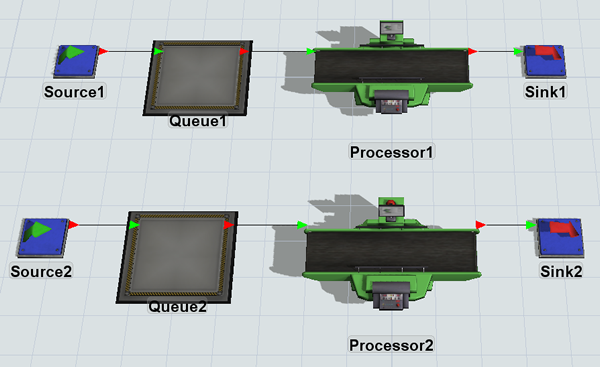
To make these changes:
- In the 3D model, hold down the Shift key and draw a box around Source1, Queue1, Processor1, and Sink1 to select them.
- Press Ctrl+C to copy the objects.
- Press Ctrl+V to paste copies of the objects.
- Press the Shift key and click on a blank area in the model to de-select the objects.
- For clarity, rename the copied objects so that they all have a 2 after them, such as Source2, Queue2, etc.
- Click Processor2 to select it.
- In Quick Properties under the Processor group, next to
the Process Time box, click the Edit
Properties button
 to open
the distribution chooser.
to open
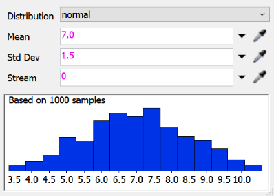
the distribution chooser. - Change the Mean to
7.0and the Standard Deviation to1.5. - Click outside this window to save the changes.
Consider saving your model.
Step 2 Add the Second Processor to the Collector
In this step, you'll learn how to add the second processor to the ProcessingTimes collector. You'll run your model to see how this affects your data table and charts.
To add the second processor:
- In the Toolbox under Statistics Collectors, double-click the ProcessingTimes collector to open its properties.
- In the Event Listening tab, click the
Sampler button
 to enter sampling mode.
 - Click Processor2 to open a menu. Select On Staytime Change to sample this event.
- In the Event Details group, click the Change Rule menu and select Update.
- In the Parameters table, change the Label Name of the New Value parameter to ItemStaytime.
- Click the Apply button to save the changes.
- On the General tab, click the View Table button to open the data table.
- On the simulation control bar, click the arrow next to Run Speed to open its properties. In the Custom box, type 10 and click the Set button.
- Reset and run the model.
As you watch the model run, notice that now flow items from both processors add staytime data to the data table, but that the data table doesn't distinguish between which processor is associated with each flow item. Also notice that now both processors update the histogram. If you were to run the simulation model at a faster speed, you'd notice that this would skew the bell curve a bit because they are using slightly different means and standard deviations:
Step 3 Separate Objects in the Collector
In this step, you'll learn how to make the statistics collector distinguish between different objects. To make this distinction, you'll add a column to the data table that records which processor is associated with each staytime event. You'll also update the histogram chart to use this column to distinguish between the two processors' staytimes.
To make these changes:
- Open the ProcessingTimes statistics collector if it's not open already.
- In the Data Recording tab, in the
Columns group, click the Add
button
 .
. - In the Name box, change the column's name to Object.
- Click the arrow next to the Value box to open a menu. Point to IDs, then select ID of Event Object.
- Confirm that the Display Format menu is set to Object.
- Click the OK button to save the changes and close the window.
- In the Dashboard, double-click the Processing Times histogram to open its properties. Notice that the properties now show the new Object column you just created.
- In the Data tab in the Split Data by table, check the Object checkbox.
- In the Settings tab, in the Bucket Count box, change the number to 20.00.
- Click the OK button to save the changes and close the window.
- Reset and run the model.
Now as you watch the model run, notice that your data table has two columns, with a new column indicating which processor processed the flow item.
Also notice that both processors gradually begin to show up as two different bell curves on the histogram, consistent with their individual distribution settings.
Step 4 Add Objects to Groups
In this step, you'll start by adding a third set of objects to the model. You'll modify the processing time of the newest processor so that it uses a different bell curve distribution. Then you'll create two groups: one for all the processors in the model and one for all the queues. Be aware that you won't use the queue group until you get to the next tutorial task, but it's easier to go ahead and make that group now in this step.
To make these changes:
- In the 3D model, hold down the Shift key and draw a box around Source1, Queue1, Processor1, and Sink1 to select them.
- Press Ctrl+C to copy the objects.
- Press Ctrl+V to paste copies of the objects.
- Press the Shift key and click on a blank area in the model to de-select the objects.
- For clarity, rename the copied objects so that they all have a 3 after them, such as Source3, Queue3, etc.
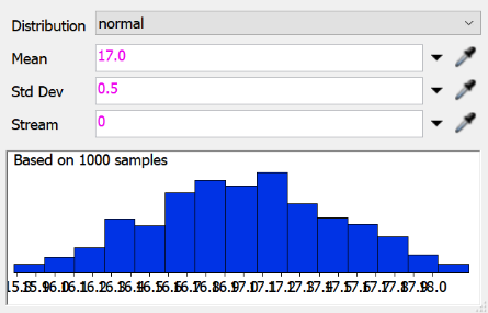
- Click Processor3 to select it.
- In Quick Properties under the Processor group, next to
the Process Time box, click the Edit
Properties button to open
the Distribution Chooser.
- Change the Mean to
17.0and the Standard Deviation to0.5. - In the Toolbox, click the Add button
to open a menu. Select
Group.
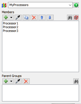
- In the name box at the top of the window, change the name of the group to MyProcessors.
- Click the Sampler button to enter sampling mode. Click Processor1 to add it to the group.
- Repeat the previous step to add Processor2 and Processor3 to the MyProcessors group.
- Close the group and confirm that the MyProcessors group now shows up in the Toolbox under Groups.
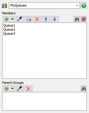
- Repeat the previous steps to create a second group called MyQueues. Add Queue1, Queue2, and Queue3 to this group.
Consider saving your simulation model.
Step 5 Add Group Events to the Collector
In this step, you'll learn how to set up a statistics collector so that it will listen to a group of objects. Listening to groups is a great way to make your model scale better. You will only have to set up a statistics collector one time to listen to a group. Then as new objects get added to the model, you can add them to that group rather than adding each individual object to the statistics collector.
To set up group listening on a statistics collector:
- In the Toolbox under Statistics Collectors, double-click the ProcessingTimes collector to open its properties window.
- On the Event Listening tab, click
Processor1 - On Staytime Change in the event list to select
it. Click the Remove button
 to delete this event.
 - Repeat the previous step to delete the Processor2 - On Staytime Change event from the event list as well. The event list will now be empty.
- Click the Sampler button to enter sampling mode.
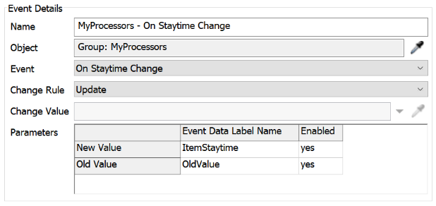
- In the Toolbox, click the MyProcessors group to open a menu. Select On Staytime Change to sample it. Notice that this event now shows up in the statistic collector's event list.
- In the Event Details group, click the Change Rule menu and select Update.
- In the Parameters table, change the Label Name of the New Value parameter to ItemStaytime.
- You'll use the same settings to create the data table that you used in previous steps, so there is no need to change anything on the Data Recording tab. Click OK to save the changes and close the model.
- Reset and run the model.
Notice that your data table includes data from all three processors in the MyProcessors group:
Also notice that the third processor now shows up as a separate bell curve on the histogram:
Step 6 Create a Timeplot Chart
In this step, you'll add a new column to the collector's data table that tracks the time an event occurs. Since this collector is listening to the staytime events for the all the processors in the simulation model, it will record the timestamp for the moment a processor finishes processing a flow item.
Once you've set up your statistics collector to track event times, you'll be able to create a timeplot chart. Like a histogram, a timeplot can show you trends in your data and can compare data from multiple objects. But one advantage of a timeplot is that it can show you peaks and troughs in the trends over time if there is an event that has a sudden impact on the trends.
The timeplot chart you'll make in this step will mark a point on a chart every time a staytime event occurs, which means each flow item will be represented by a small dot on the chart. The x-axis will represent the time (in FlexSim model units) that the flow item was finished being processed. The y-axis will represent the length of time the processor processed the flow item. Just like on the histogram, the different items that were processed by different processors will be represented by different colors.
To create this chart:
- In the Toolbox under Statistics Collectors, double-click the ProcessingTimes collector to open its properties window.
- In the Data Recording tab in the
Columns group, click the Add
button to add a new column.
- In the Name box, change the name of the column to Time.
- Click the arrow next to the Value box to open a menu. Point to Time, then select Model Date/Time.
- Click the OK button to save the changes and close the properties window.
- On the simulation control bar, press the Reset button to refresh the model.
- Double-click in a blank space in the dashboard to open the Quick Library.
- Under the Charts group, click the Time Plot chart to add it to the dashboard. Its properties window will open automatically.
- In the name box at the top of the window, change the display name of the chart to Processor Staytimes.
- Click the Data Source menu and select the ProcessingTimes collector.
- In the Data tab, click the X Values menu and select Time.
- Click the Y Values menu and select Staytime.
- In the Split Data By group, check the Object checkbox.
- Click the OK button to save the changes and close the window.
- Reset and run the model.
Notice that your data table now includes the time the item was finished being processed by the processor:
Using the time information, the new timeplot chart creates a point on the timeplot for each flow item as it is processed by processors. Notice that you can see clear trendlines in the three processors' staytimes:
Conclusion
Now that you've finished this tutorial task, you likely have a good sense of how you can use a statistics collector to track and compare data from multiple objects. In the next tutorial task, you'll learn how to use a calculated table with a statistics collector to create custom statistics. Continue on to Tutorial Task 2.3 - Create and Track Custom Statistics.