Task Overview

For this tutorial, let us examine a very simple situation. A single worker must carry an item from a source to a processor. After the item finishes processing, the worker must carry it to a second processor that takes longer than the first. After the the second processor finishes the item, the worker then carries it to the sink.

Now we want to see if we can maximize the throughput of this system by adjusting (which is also tied to revenue) the position of the processors. If each processor could be moved up to three meters right or left, where should each be placed? It would be very difficult to intuitively know how to place both processors to maximize throughput. In order to solve this problem accurately, we will use the Experimenter and Optimizer.

Obviously this is a drastically simplified scenario, but often in real life you have situations where you want to see how various layouts affect overall throughput. This is a very simplistic implementation of such an experiment.

Step 1 Build the 3D Model

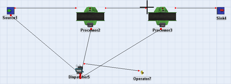
In this step, you'll build a basic 3D model for this tutorial. When you're finished, your model should look similar to the following image:

To build this model:

1. Make sure your 3D model window is open and active. From the Library, drag the following 3D objects into the model:
   • A Source
   • A Processor
   • A Processor
   • A Sink
   • A Dispatcher
   • An Operator
2. Set the location of the objects according to the table below:

   Object	X Position	Y Position
   Source1	-20.0	0.0
   Processor2	-10.0	0.0
   Processor3	0.0	0.0
   Sink4	10.0	0.0
   Dispatcher5	N/A	N/A
   Operator7	N/A	N/A

   Dispatcher5 and Operator7 do not need to be in a particular place, but they should not be in line with the rest of the objects.
3. Set the following logic:
   • Set Source1, Processor2, and Processor3 to Use Transport.
   • Set the process time of Processor2 to normal(10, 2).
   • Set the process time of Processor3 to normal(12, 3).
   • Set the reset position of Operator7 to its current position.

Check to ensure your model looks similar to the image shown at the beginning of this step.

Step 2 Creating Variables

Open the Experimenter window by selecting it from the Statistics menu of the Toolbox. Position the window so you can see the processors in the model as well as the window. Then, for Processor2 and then Processor3, follow these steps:

1. • Click on the processor in the 3D view.
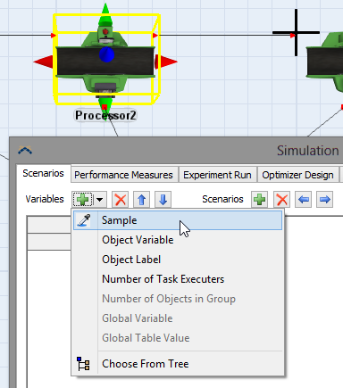
   • Click on the Position button in the Quick Properties and set the position reference to Direct Spatials.
   • Click the down arrow on the button.
   • Select Sample from the popup menu. This puts the cursor in sample mode.

   

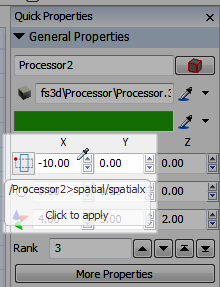
2. Sample the X position field in the Quick Properties menu by clicking on it. This adds a new experiment variable.

   

3. Set the value of Scenario 1 for the new variable by double-clicking the cell and entering the new value.

   

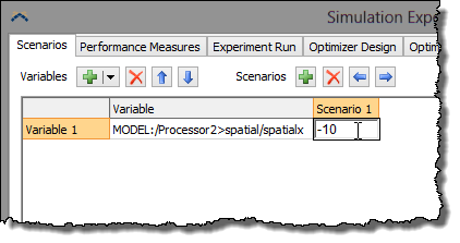
4. Set the name of the variable by double-clicking on the current name. Set the name to Proc2X for Processor2 and Proc3X for Processor3.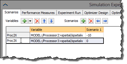

   

Step 3 Creating Performance Measures

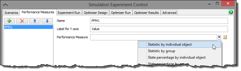
1. Go to the Performance Measures tab in the Experimenter window. From there:

   • Click the button to add a new performance measure.
   • Name the new performance measure Throughput.
   • Click the button and select the first option. A popup will appear.

   

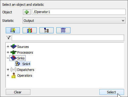
2. Select Sink4 for the object and Input for the statistic. To select the object simply type Sink4 in the object field or do the following:

   • Click the button.
   • Select Sink4 from the list of objects.
   • Click the Select button when you are finished.

   

Step 4 Designing the Experiment

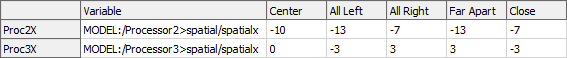
Now that we've created the variables and performance measures, we'll set up some scenarios for our experiment.

1. Go back to the Scenarios tab.
2. Create 5 scenarios by clicking on the Scenarios button 4 times.

3. Enter scenario names and values as follows:

   

Step 5 Running the Experiment

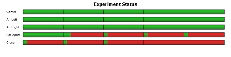
Go to the Experiment Run tab. Hit the button. Each scenario will be run 5 times and the results of the Throughput performance measure will be collected at the end of each run. The status window will show which scenarios/replications are currently being run. FlexSim will run multiple scenarios simultaneously if your computer has a multi-core cpu.

Once the experiment is finished, click the button at the bottom. This will open a window where you can get data on the performance measures for the scenario. In this example we only have one performance measure, but if you had multiple you could see the results for each in this window. There are several options for how to display the data, including a Replications Plot, a Frequency Histogram, a Correlation Plot (for examining correlations between multiple performance measures), a Data Summary, and a Raw Data view.

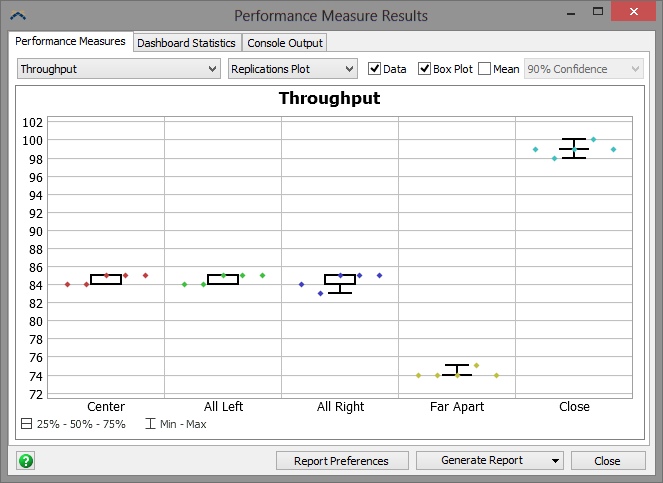
In this experiment, the best scenario was the "Close" scenario, which averaged right around 99 parts of throughput. The worst scenario was the "Far Apart" scenario, which averaged about 75 parts throughput.

Conclusion

At this point, you've learned how to use the Experimenter. In the next tutorial task, you'll learn how to use the Optimizer. Continue on to Tutorial Task 4.2 - Optimizer.