Empirical Distribution
Overview and Key Concepts
The Empirical Distribution tool is used to generate random values given a table of empirical data:
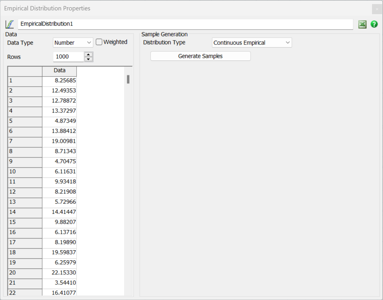
The Empirical Distribution tool provides a table. This table is an input to the tool. The table should contain historical or typical values. You can then treat the Empirical Distribution tool as a random distribution function. It will generate random values based on the input data so that the random values will match the same distribution as the input values.
The Empirical Distribution tool is accessed from the Toolbox.
Data Types
The Empirical Distribution tool supports either Number or String (text) values. If you use text values, the tool will automatically set the Distribution Type to Discrete.
Value Weights
If you check the Weighted box, you'll be able to supply weights for each value. If you don't check the box, all values will be given an identical default weight. n either case, the Empirical Distribution tool sorts the input values and combines duplicate values and their weights.
The end result is that you can increase the likelihood of a value (or, for Continuous data, nearby values) by increasing the total weight of a given value. You can increase total weight by specifying weight directly or by adding more instances of the value to the table.
Data Input
You can set values in the input table either manually or through the Excel Interface. Data does not have to be in any order. For more information about importing data from Excel, see the Excel Interface topic.
Sample Generation
The Sample Generation pane lets you define how random samples will be generated from the empirical data.
See Empirical Distribution API for more information on how to generate a random variate from the Empirical Distribution tool. If a field accepts random distributions, there is usually a picklist option available to use an Empirical Distribution too.
Selecting Distribution Type
You can set the Distribution Type to one of the following values:
- Continuous Empirical
- Discrete Empirical
- Fitted Distribution
Continuous Empirical
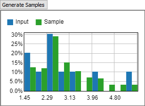
When set to Continuous Empirical, the tool assumes the values in the table come from a continuous distribution, such as a process time. When sampling from the tool, it can return any value between the minimum and maximum values. The tool is unlikely to return any particular input value. However, the distribution of returned values will match the distribution of input values. Using a Continuous distribution is a good choice for process time data.
You can use the Generate Samples button to display a histogram showing both the input data and sampled random data.
Discrete Empirical
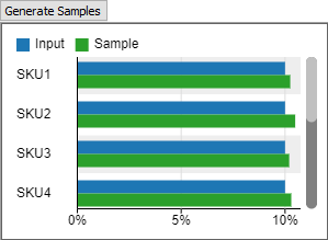
When set to Discrete Empirical, the tool assumes that the values in the table form the complete set of possible values. When sampling from the tool, it will return one of the values given in the table. The likelihood of a given value is determined by its frequency or weight in the input data. Using a Discrete distribution is a good choice for discrete values, such as the number of items in an order, or for choosing a random SKU.
You can use the Generate Samples button to display a bar chart showing both the input data and sampled random data.
Fitted Distribution
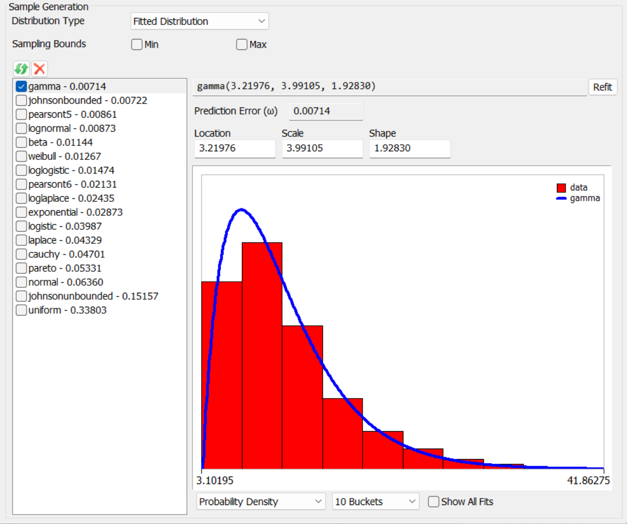
When set to Fitted Distribution, the tool shows additional buttons and controls that let you fit the data to existing distributions. When sampling from the tool, it will generate random samples from the fitted distribution you choose.
Press the 
Each fit shows the name of the distribution, its fitted parameters, and a Prediction Error (ω). This is a score, between 0 and 1, that tells how good the fit is to the data. Lower numbers are better.
There are also controls below the fit graph that let you show either a probability density function or a cumulative distribution function, a number of buckets, etc.
Defining Min and Max
Since many distributions have long tails or may not always return positive values, the tool also allows you to define a Min and Max value. This lets you define a specific range of values within which generated samples must remain. Check the appropriate box and enter the desired min or max value for sampling. When these are defined, the tool will repeatedly resample from the fitted distribution until the sample falls within the min/max range.
Curve Fitting Algorithm
FlexSim uses a relatively simple curve fitting algorithm for fitting data to parameterized probability distributions. Note that FlexSim's curve fitter is not intended to be used for full statistical analysis of various curve fits. For that, there are several off-the-shelf distribution fitters that you can purchase, such as ExpertFit, Stat::Fit, scipy.optimize.curve_fit, etc. In our experience many datasets do not fit well to any known distributions, so we advise users to resample the data directly using the Continuous Empirical option, which is the default option for the Empirical Distribution tool. Nevertheless, FlexSim's curve fitting features can be helpful in some scenarios. In the interest of transparency, we document here the algorithms that are used for fitting data to various distributions.
FlexSim's curve fitter mixes using generally known maximum likelihood estimators (MLEs) with optimization principles to find distribution parameters that best fit the data. For each distribution family, there are usually some known maximum likelihood estimators for the parameters. For example, the MLE for the normal distribution's μ parameter is the sample mean, and the MLE for its σ parameter is the sample standard deviation. Where these MLEs are known, we simply calculate the MLE and use that as the 'best fit' for the data. We have primarily used Simulation Modeling & Analysis, 5th Edition by Averill Law to find known MLE calculations.
For some distribution families, there are parameters which do not have known (at least to us) MLE calculations. Sometimes these are additional parameters to the random number generation functions, such as location, which are not part of the standard definitions for these distribution families, or sometimes their MLE calculations are simply not documented. We refer to these as the non-MLE parameters. For the non-MLE parameters, FlexSim's curve fitter makes an initial guess at the value, and then runs an iterative gradient descent algorithm to find values that best fit the curve.
Gradient Descent
As the objective function for the gradient descent algorithm, the fitter performs a
Cramér-von Mises goodness of fit test, and uses the resulting
$\large{T} = \large{n \omega^2} = \Large{\frac{1}{12 n} + \sum\limits_{i=1}^{n}[\frac{2i - 1}{2n} - F(x_i)]^2 }$
The minimization objective, and the value that is shown as a 'fit score' in the UI, is ω.
$\large{\omega} = \Large{\sqrt{\frac{T}{n}}}$
ω will always be a value between 0 and 1, with lower values signifying a better fit.
At each iteration, the gradient descent algorithm first gets the objective with the current parameters. It then calculates a partial gradient for each non-MLE parameter by slightly adjusting that parameter and reevaluating the objective. Then it combines the partial gradients into a cumulative gradient, steps in the direction of the gradient, and then repeats the process.
The step size of the gradient descent is adjusted as the algorithm progresses. The step size starts at a value of 1, and the algorithm keeps track of the gradient of the last iteration. At each iteration, after determining the new gradient, it calculates the dot product of the current gradient with the last gradient, which represents the cosine of the angle between the two vectors. If this value is near 1 — the current gradient is close to the same as the last gradient — then the step size is increased. If the value is close to zero — the gradient has changed significantly — then the step size decreases. The end effect is that the algorithm will gain momentum as it travels in the same direction, but will slow down as it begins to circle around a minimum.
The algorithm proceeds until either a maximum number of iterations is executed, or the step size decreases to a minimum threshold.
Disclaimers
FlexSim's curve fitter does not perform hypothesis testing on whether the data came from the fitted distribution. It only performs the gradient descent that minimizes ω, and then shows the parameters and the resulting ω. It also lets you see graphs that compare either a histogram of the data with the distribution's probability density function, or the data's empirical distribution function with the distribution's cumulative distribution function. We also assume that the data that is being fitted is continuous, and thus only fit to continuous distributions. Further, the curve fitter will naturally suffer the standard deficiencies associated with gradient descent: solutions may resolve to local minima. Again, for robust full-featured curve fitting there are many third-party solutions available.